2. GSEApy Tutorial
GSEApy is a Python/Rust toolkit for Gene Set Enrichment Analysis and related methods. This notebook walks through every public entry point with small, runnable demos using the data bundled in the repository’s tests/ folder.
2.1. What this notebook covers
Section |
Function |
What it does |
|---|---|---|
|
— |
imports and version check |
|
|
convert gene IDs, map orthologs between species |
|
|
download MSigDB gene-set collections ( |
|
|
list / fetch Enrichr gene-set libraries |
|
|
Enrichr web service |
|
|
local hypergeometric test |
|
|
GSEA on a single ranked list |
|
|
phenotype-permutation GSEA |
|
|
single-sample GSEA |
|
|
gene set variation analysis |
|
|
re-plot results from the Broad GSEA Java app |
Tip: run the cells in order. Sections 2–5 call online services (Biomart, MSigDB, Enrichr) and need an internet connection; everything else runs fully offline on the bundled test data.
2.1.1. Setup
Import GSEApy together with pandas and matplotlib. The two %autoreload magics are only useful if you are editing the GSEApy source while you work — they reload changed modules automatically. They are harmless otherwise.
[1]:
# %matplotlib inline
# %config InlineBackend.figure_format = 'retina'  # crisper figures on HiDPI/Mac screens
%load_ext autoreload
%autoreload 2

import pandas as pd
import matplotlib.pyplot as plt
import gseapy as gp
Check the installed GSEApy version (this tutorial targets v1.x).
[2]:
gp.__version__
[2]:
'1.3.0'
2.1.2. Biomart API
Biomart is a thin client over the Ensembl BioMart web service. Use it to convert gene identifiers (Ensembl ID ↔ gene symbol ↔ Entrez ID) and to map orthologs between species.
Note: BioMart support is limited and the public server can be slow or occasionally unavailable. Skip this section if you do not need ID conversion.
2.2. Convert gene identifiers
[3]:
from gseapy import Biomart

bm = Biomart()
[4]:
# The commented helpers below let you discover valid marts/datasets/attributes/filters.
# Run them once to explore, then build your real query.
# marts    = bm.get_marts()                                   # available marts
# datasets = bm.get_datasets(mart='ENSEMBL_MART_ENSEMBL')     # datasets in a mart
# attrs    = bm.get_attributes(dataset='hsapiens_gene_ensembl')  # columns you can request
# filters  = bm.get_filters(dataset='hsapiens_gene_ensembl')     # columns you can filter on

# A query needs: a dataset, the attributes (columns) to return, and optional filters.
# `filters` must be a dict mapping a filter name to the values to keep.
queries = {'ensembl_gene_id': ['ENSG00000125285', 'ENSG00000182968']}

results = bm.query(
    dataset='hsapiens_gene_ensembl',
    attributes=['ensembl_gene_id', 'external_gene_name', 'entrezgene_id', 'go_id'],
    filters=queries,
)
results.tail()
[4]:
| ensembl_gene_id | external_gene_name | entrezgene_id | go_id | |
|---|---|---|---|---|
| 27 | ENSG00000182968 | SOX1 | 6656 | GO:0007420 |
| 28 | ENSG00000182968 | SOX1 | 6656 | GO:0030182 |
| 29 | ENSG00000182968 | SOX1 | 6656 | GO:0043565 |
| 30 | ENSG00000182968 | SOX1 | 6656 | GO:0048713 |
| 31 | ENSG00000182968 | SOX1 | 6656 | GO:1904936 |
Inspect the column types of the returned table.
[5]:
results.dtypes
[5]:
ensembl_gene_id       object
external_gene_name    object
entrezgene_id          Int32
go_id                 object
dtype: object
2.3. Map gene symbols between mouse and human
This is handy when you need to translate gene symbols across species — for example, to run a human gene-set library against mouse data. We pull the full ortholog mapping in both directions (no filter ⇒ all genes), so each query returns the whole genome and may take a little while.
[6]:
from gseapy import Biomart

bm = Biomart()

# Mouse -> Human orthologs. Note the dataset and attribute names differ per direction.
m2h = bm.query(
    dataset='mmusculus_gene_ensembl',
    attributes=['ensembl_gene_id', 'external_gene_name',
                'hsapiens_homolog_ensembl_gene',
                'hsapiens_homolog_associated_gene_name'],
)

# Human -> Mouse orthologs.
h2m = bm.query(
    dataset='hsapiens_gene_ensembl',
    attributes=['ensembl_gene_id', 'external_gene_name',
                'mmusculus_homolog_ensembl_gene',
                'mmusculus_homolog_associated_gene_name'],
)
[7]:
# Peek at a random sample of the human -> mouse mapping.
h2m.sample(5)
[7]:
| ensembl_gene_id | external_gene_name | mmusculus_homolog_ensembl_gene | mmusculus_homolog_associated_gene_name | |
|---|---|---|---|---|
| 79602 | ENSG00000105750 | ZNF85 | ENSMUSG00000048280 | Zfp738 |
| 85423 | ENSG00000137135 | ARHGEF39 | ENSMUSG00000051517 | Arhgef39 |
| 71287 | ENSG00000137077 | CCL21 | ENSMUSG00000094065 | Ccl21d |
| 20341 | ENSG00000306096 | NaN | NaN | NaN |
| 5195 | ENSG00000273092 | TAS2R20 | NaN | NaN |
2.4. Translate a .gmt gene-set file to another species
GSEApy gene symbols are case-sensitive when used offline, and most public libraries (Enrichr, MSigDB) ship human symbols. To run them against mouse data, convert the gene members with the ortholog map built above.
Example: convert a human KEGG library to mouse symbols.
[8]:
# Build a {human_symbol: mouse_symbol} lookup, dropping rows with missing values.
h2m_dict = {}
for _, row in h2m[['external_gene_name', 'mmusculus_homolog_associated_gene_name']].iterrows():
    if row.isna().any():
        continue
    h2m_dict[row['external_gene_name']] = row['mmusculus_homolog_associated_gene_name']

# Read a human KEGG .gmt into a {term: [genes]} dict.
kegg = gp.read_gmt(path="tests/extdata/enrichr.KEGG_2016.gmt")
print("Human symbols:", kegg['MAPK signaling pathway Homo sapiens hsa04010'][:10])
Human symbols: ['EGF', 'IL1R1', 'IL1R2', 'HSPA1L', 'CACNA2D2', 'CACNA2D1', 'CACNA2D4', 'CACNA2D3', 'MAPK8IP3', 'MAPK8IP1']
[9]:
# Translate every gene in every term to its mouse ortholog (skip genes with no mapping).
kegg_mouse = {}
for term, genes in kegg.items():
    kegg_mouse[term] = [h2m_dict[g] for g in genes if g in h2m_dict]

print("Mouse symbols:", kegg_mouse['MAPK signaling pathway Homo sapiens hsa04010'][:10])
Mouse symbols: ['Egf', 'Il1r1', 'Il1r2', 'Hspa1l', 'Cacna2d2', 'Cacna2d1', 'Cacna2d4', 'Cacna2d3', 'Mapk8ip3', 'Mapk8ip1']
2.4.1. MSigDB API
Msigdb downloads gene-set collections from the MSigDB (Broad Institute). You pick a category (e.g. hallmark, curated, GO) and a database version (dbver), and get back a {term: [genes]} dict ready to pass to any GSEApy function.
[10]:
from gseapy import Msigdb

msig = Msigdb()
# Mouse hallmark gene sets (category 'mh.all') from the 2023.1.Mm release.
gmt = msig.get_gmt(category='mh.all', dbver="2023.1.Mm")
Two helpers let you discover valid values before downloading:
msig.list_dbver()                  # list available database versions
msig.list_category(dbver="2023.1.Hs")  # list categories for a given version
[11]:
# Inspect one hallmark set.
print(gmt['HALLMARK_WNT_BETA_CATENIN_SIGNALING'])
['Ctnnb1', 'Jag1', 'Myc', 'Notch1', 'Ptch1', 'Trp53', 'Axin1', 'Ncstn', 'Rbpj', 'Psen2', 'Wnt1', 'Axin2', 'Hey2', 'Fzd1', 'Frat1', 'Csnk1e', 'Dvl2', 'Hey1', 'Gnai1', 'Lef1', 'Notch4', 'Ppard', 'Adam17', 'Tcf7', 'Numb', 'Ccnd2', 'Ncor2', 'Kat2a', 'Nkd1', 'Hdac2', 'Dkk1', 'Wnt5b', 'Wnt6', 'Dll1', 'Skp2', 'Hdac5', 'Fzd8', 'Dkk4', 'Cul1', 'Jag2', 'Hdac11', 'Maml1']
2.4.2. Enrichr gene-set libraries
Enrichr hosts hundreds of curated gene-set libraries. GSEApy can list them and download any of them as a {term: [genes]} dict for use with enrichr, enrich, prerank, gsea, ssgsea, or gsva.
List the available library names.
Choose the organism from: 'Human', 'Mouse', 'Yeast', 'Fly', 'Fish', 'Worm'.
[12]:
# Default organism is Human.
names = gp.get_library_name()
names[:10]
[12]:
['ARCHS4_Cell-lines',
 'ARCHS4_IDG_Coexp',
 'ARCHS4_Kinases_Coexp',
 'ARCHS4_TFs_Coexp',
 'ARCHS4_Tissues',
 'Achilles_fitness_decrease',
 'Achilles_fitness_increase',
 'Aging_Perturbations_from_GEO_down',
 'Aging_Perturbations_from_GEO_up',
 'Allen_Brain_Atlas_10x_scRNA_2021']
[13]:
# Library names differ per organism.
yeast = gp.get_library_name(organism='Yeast')
yeast[:10]
[13]:
['Cellular_Component_AutoRIF',
 'Cellular_Component_AutoRIF_Predicted_zscore',
 'GO_Biological_Process_2018',
 'GO_Biological_Process_AutoRIF',
 'GO_Biological_Process_AutoRIF_Predicted_zscore',
 'GO_Cellular_Component_2018',
 'GO_Cellular_Component_AutoRIF',
 'GO_Cellular_Component_AutoRIF_Predicted_zscore',
 'GO_Molecular_Function_2018',
 'GO_Molecular_Function_AutoRIF']
Download a library into a ``{term: [genes]}`` dict.
[14]:
# Fetch one library by name (or pass a local .gmt path to read_gmt instead).
go_mf = gp.get_library(name='GO_Molecular_Function_2018', organism='Yeast')
print(go_mf['ATP binding (GO:0005524)'])
['MLH1', 'ECM10', 'RLI1', 'SSB1', 'SSB2', 'MSH2', 'YTA12', 'CDC6', 'HMI1', 'YNL247W', 'MSH6', 'SSQ1', 'MCM7', 'SRS2', 'HSP104', 'SSA1', 'MCX1', 'SSC1', 'ARP2', 'ARP3', 'SSE1', 'SMC2', 'SSZ1', 'TDA10', 'ORC5', 'VPS4', 'RBK1', 'NEW1', 'SSA4', 'ORC1', 'KAR2', 'SSA2', 'DYN1', 'SSA3', 'PGK1', 'VPS33', 'LHS1', 'CDC123', 'PMS1']
2.4.3. Over-representation analysis (Enrichr web service)
gp.enrichr() sends a gene list to the Enrichr web service and returns enrichment results. The only required input is a list of gene symbols.
Accepted inputs
gene_list: alist,pandas.Series, single-columnDataFrame, or a.txtfile with one gene symbol per line.gene_sets: one or more Enrichr library names (comma-separated string or list), a local.gmtpath, or a{term: [genes]}dict.
gene_list = "./data/gene_list.txt"      # or a Python list / Series
gene_sets = "KEGG_2016"                  # one library
gene_sets = "KEGG_2016,KEGG_2013"        # several, comma-separated
gene_sets = ["KEGG_2016", "KEGG_2013"]   # several, as a list
Note: for the online service, gene symbols are not case-sensitive — they are upper-cased automatically.
[15]:
# Load an example gene list (one symbol per line).
gene_list = pd.read_csv("./tests/data/gene_list.txt", header=None, sep="\t")
gene_list.head()
[15]:
| 0 | |
|---|---|
| 0 | IGKV4-1 |
| 1 | CD55 |
| 2 | IGKC |
| 3 | PPFIBP1 |
| 4 | ABHD4 |
[16]:
# A DataFrame/Series can be flattened to a plain Python list if you prefer.
glist = gene_list.squeeze().str.strip().to_list()
print(glist[:10])
['IGKV4-1', 'CD55', 'IGKC', 'PPFIBP1', 'ABHD4', 'PCSK6', 'PGD', 'ARHGDIB', 'ITGB2', 'CARD6']
2.5. Enrichr without a custom background
Set outdir=None to keep results in memory only (nothing written to disk). The returned object stores the table on both .res2d (last query) and .results (all queries).
[17]:
enr = gp.enrichr(
    gene_list=gene_list,                              # or "./tests/data/gene_list.txt"
    gene_sets=['MSigDB_Hallmark_2020', 'KEGG_2021_Human'],
    organism='human',                                 # set to your organism, e.g. 'Yeast'
    outdir=None,                                       # keep results in memory only
)
[18]:
# All enrichment results across the requested libraries.
enr.results.head(5)
[18]:
| Gene_set | Term | Overlap | P-value | Adjusted P-value | Old P-value | Old Adjusted P-value | Odds Ratio | Combined Score | Genes | |
|---|---|---|---|---|---|---|---|---|---|---|
| 0 | MSigDB_Hallmark_2020 | IL-6/JAK/STAT3 Signaling | 19/87 | 1.197225e-09 | 5.986123e-08 | 0 | 0 | 6.844694 | 140.612324 | IL4R;TGFB1;IL1R1;IFNGR1;IL10RB;ITGB3;IFNGR2;IL... |
| 1 | MSigDB_Hallmark_2020 | TNF-alpha Signaling via NF-kB | 27/200 | 3.220898e-08 | 5.368163e-07 | 0 | 0 | 3.841568 | 66.270963 | BTG2;BCL2A1;PLEK;IRS2;LITAF;IFIH1;PANX1;DRAM1;... |
| 2 | MSigDB_Hallmark_2020 | Complement | 27/200 | 3.220898e-08 | 5.368163e-07 | 0 | 0 | 3.841568 | 66.270963 | FCN1;LRP1;PLEK;LIPA;CA2;CASP3;LAMP2;S100A12;FY... |
| 3 | MSigDB_Hallmark_2020 | Inflammatory Response | 24/200 | 1.635890e-06 | 2.044862e-05 | 0 | 0 | 3.343018 | 44.540108 | LYN;IFITM1;BTG2;IL4R;CD82;IL1R1;IFNGR2;ITGB3;F... |
| 4 | MSigDB_Hallmark_2020 | heme Metabolism | 23/200 | 5.533816e-06 | 5.533816e-05 | 0 | 0 | 3.181358 | 38.509172 | SLC22A4;MPP1;BNIP3L;BTG2;ARHGEF12;NEK7;GDE1;FO... |
2.6. Enrichr with a custom background
Provide your own background gene list (e.g. all genes expressed in your assay).
Note: when a background is supplied, the output omits the
Overlapcolumn.
[19]:
enr_bg = gp.enrichr(
    gene_list=gene_list,
    gene_sets=['MSigDB_Hallmark_2020', 'KEGG_2021_Human'],
    background="tests/data/background.txt",            # the 'organism' arg is ignored when set
    outdir=None,
)
[20]:
enr_bg.results.head()
[20]:
| Gene_set | Term | P-value | Adjusted P-value | Old P-value | Old adjusted P-value | Odds Ratio | Combined Score | Genes | |
|---|---|---|---|---|---|---|---|---|---|
| 0 | MSigDB_Hallmark_2020 | IL-6/JAK/STAT3 Signaling | 3.559435e-11 | 1.779718e-09 | 0 | 0 | 8.533251 | 205.300064 | IL4R;TGFB1;IL1R1;IFNGR1;IL10RB;ITGB3;IFNGR2;IL... |
| 1 | MSigDB_Hallmark_2020 | TNF-alpha Signaling via NF-kB | 3.401526e-10 | 6.356588e-09 | 0 | 0 | 4.824842 | 105.189414 | BTG2;BCL2A1;PLEK;IRS2;LITAF;IFIH1;PANX1;DRAM1;... |
| 2 | MSigDB_Hallmark_2020 | Complement | 3.813953e-10 | 6.356588e-09 | 0 | 0 | 4.796735 | 104.027683 | FCN1;LRP1;PLEK;LIPA;CA2;CASP3;LAMP2;S100A12;FY... |
| 3 | MSigDB_Hallmark_2020 | Inflammatory Response | 3.380686e-08 | 4.225857e-07 | 0 | 0 | 4.197067 | 72.200480 | LYN;IFITM1;BTG2;IL4R;CD82;IL1R1;IFNGR2;ITGB3;F... |
| 4 | MSigDB_Hallmark_2020 | heme Metabolism | 8.943634e-08 | 8.943634e-07 | 0 | 0 | 4.111306 | 66.725423 | SLC22A4;MPP1;BNIP3L;BTG2;ARHGEF12;NEK7;GDE1;FO... |
2.6.1. Over-representation analysis (offline hypergeometric test)
gp.enrich() runs the same over-representation test locally — it does not call the Enrichr web service. Use it for custom or private gene sets, or when you have no internet access.
Important
Input gene symbols are case-sensitive here.
The identifier type in your
gene_listmust match the one used in the gene sets (.gmt/dict).
gene_setsaccepts a.gmtpath or a{term: [genes]}dict:gene_sets = "./data/genes.gmt" gene_sets = {'A': ['gene1', 'gene2', ...], 'B': ['gene2', 'gene4', ...]}
[21]:
# Note: the offline function is `enrich` (no trailing "r"), unlike the online `enrichr`.
# gene_sets here mixes a .gmt file, a name that won't resolve ("unknown"), and a dict (kegg).
enr2 = gp.enrich(
    gene_list="./tests/data/gene_list.txt",           # or a Python list
    gene_sets=["./tests/data/genes.gmt", "unknown", kegg],
    background=None,    # None | int | gene list | text file | a Biomart dataset name
    outdir=None,
    verbose=True,
)
2026-06-24 11:23:41,352 [INFO] User defined gene sets is given: ./tests/data/genes.gmt
2026-06-24 11:23:41,356 [INFO] Input dict object named with gs_ind_2
2026-06-24 11:23:41,735 [WARNING] Input library not found: unknown. Skip
2026-06-24 11:23:41,736 [INFO] Off-line enrichment analysis with library: genes.gmt
2026-06-24 11:23:41,738 [INFO]   Background is not set! Use all 682 genes in genes.gmt.
2026-06-24 11:23:41,743 [INFO] Off-line enrichment analysis with library: gs_ind_2
2026-06-24 11:23:41,768 [INFO]   Background is not set! Use all 7010 genes in gs_ind_2.
2026-06-24 11:23:41,791 [INFO] Done.
[22]:
enr2.results.head()
[22]:
| Gene_set | Term | Overlap | P-value | Adjusted P-value | Odds Ratio | Combined Score | Genes | |
|---|---|---|---|---|---|---|---|---|
| 0 | genes.gmt | BvA_UpIN_A | 8/139 | 0.457390 | 0.568432 | 1.169168 | 0.914547 | PADI2;MAP3K5;IL1R1;MBOAT2;MSRB2;HAL;PCSK6;IQGAP2 |
| 1 | genes.gmt | BvA_UpIN_B | 12/130 | 0.026744 | 0.187208 | 2.275467 | 8.240477 | SUOX;MBNL3;LPAR1;ST3GAL6;DYSF;FAM65B;HEBP1;ARH... |
| 2 | genes.gmt | CvA_UpIN_A | 1/12 | 0.481190 | 0.568432 | 2.334966 | 1.708011 | MBOAT2 |
| 3 | genes.gmt | DvA_UpIN_A | 16/284 | 0.426669 | 0.568432 | 1.134623 | 0.966412 | VNN1;NMNAT1;PADI2;MAP3K5;ATP6V1B2;IL1R1;KIF1B;... |
| 4 | genes.gmt | DvA_UpIN_D | 13/236 | 0.487227 | 0.568432 | 1.088533 | 0.782682 | FAM198B;MBNL3;LPAR1;ST3GAL6;DYSF;GNB4;FAM65B;T... |
2.7. Choosing a background for the offline test
By default, all genes in ``gene_sets`` are used as the background. A more accurate background is usually one of the following:
(Recommended) A list of background genes,
['gene1', 'gene2', ...]— typically the genes detectable in your experiment (e.g. expressed genes from your RNA-seq). The identifier type must match the gene sets.A total gene count, e.g.
20000. Simple, but it assumes every gene set gene is present in the background; genes in the sets but missing from the background still distort the test.A BioMart dataset name, e.g.
"hsapiens_gene_ensembl". GSEApy fetches all annotated genes for that dataset and uses them as the background.
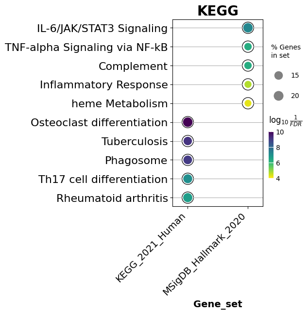
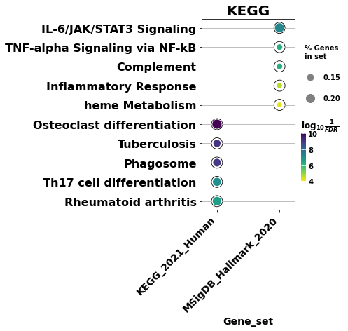
2.8. Plotting enrichment results
dotplot and barplot summarize an enrichment table. Below we show the top 5 terms per library, ranked by adjusted p-value.
[23]:
from gseapy import barplot, dotplot
[24]:
# Dot plot: dot size encodes gene overlap, color encodes significance.
# Setting x='Gene_set' faces the plot by library so you can compare them side by side.
ax = dotplot(
    enr.results,
    column="Adjusted P-value",
    x='Gene_set',          # split the x-axis by library (multi-library comparison)
    size=5,
    top_term=5,
    figsize=(3, 5),
    title="KEGG",
    xticklabels_rot=45,    # rotate x tick labels for readability
    show_ring=True,        # set False to remove the outer ring around dots
    marker='o',
)
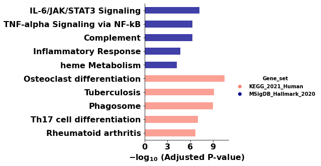
[25]:
# Bar plot grouped by library, with an explicit color per group.
ax = barplot(
    enr.results,
    column="Adjusted P-value",
    group='Gene_set',      # group bars by library (multi-library comparison)
    size=5,
    top_term=5,
    figsize=(3, 5),
    color={'KEGG_2021_Human': 'salmon', 'MSigDB_Hallmark_2020': 'darkblue'},
)
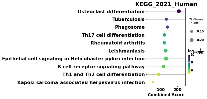
[26]:
# Single-library views use .res2d (the most recent query).
# Pass ofname='figure.pdf' to save the figure to disk.
ax = dotplot(enr.res2d, title='KEGG_2021_Human', cmap='viridis', size=5, figsize=(3, 5))
[27]:
ax = barplot(enr.res2d, title='KEGG_2021_Human', figsize=(4, 5), color='darkred')
2.9. Command-line equivalent
The same analysis is available from the gseapy enrichr CLI. The -v flag prints progress.
[28]:
# !gseapy enrichr -i ./tests/data/gene_list.txt \
#                 -g GO_Biological_Process_2017 \
#                 -v -o test/enrichr_BP
2.9.1. Preranked GSEA (prerank)
gp.prerank() runs GSEA on a single, pre-ranked gene list — for example, genes ranked by a differential-expression statistic.
Accepted ``rnk`` inputs
a 2-column
DataFrame(gene, score), or a 1-columnDataFrameindexed by genea
pandas.Seriesindexed by genea
.rnktext file (no header; anything after a#is ignored)
Accepted ``gene_sets`` inputs — same as the other functions: Enrichr library name(s), a .gmt path, or a {term: [genes]} dict.
Note on symbols: Enrichr libraries use UPPERCASE human symbols. Convert your gene identifiers to match (see Section 2.3 for cross-species conversion).
[29]:
# A .rnk file: column 0 = gene, column 1 = ranking metric.
rnk = pd.read_csv("./tests/data/temp.rnk", header=None, index_col=0, sep="\t")
rnk.head()
[29]:
| 1 | |
|---|---|
| 0 | |
| ATXN1 | 16.456753 |
| UBQLN4 | 13.989493 |
| CALM1 | 13.745533 |
| DLG4 | 12.796588 |
| MRE11A | 12.787631 |
[30]:
rnk.shape
[30]:
(22922, 1)
2.10. Run prerank
permutation_num is reduced to 1000 here to keep the demo fast. outdir=None keeps everything in memory. We use method='multilevel' (the fgsea multilevel p-value, explained just below); the default is method='permutation'.
[31]:
pre_res2 = gp.prerank(
    rnk="./tests/data/temp.rnk",   # or rnk=rnk
    gene_sets='KEGG_2016',          # Enrichr library name (downloaded automatically)
    threads=4,
    min_size=5,
    max_size=1000,
    permutation_num=1000,           # raise for publication-quality p-values
    outdir=None,
    seed=6,                         # set a seed for reproducibility
    method='multilevel',            # fgsea multilevel p-values (see below)
    verbose=True,
)
pre_res2.res2d.head(5)
2026-06-24 11:23:42,569 [WARNING] Duplicated values found in preranked stats: 4.97% of genes
The order of those genes will be arbitrary, which may produce unexpected results.
2026-06-24 11:23:42,569 [INFO] Parsing data files for GSEA.............................
2026-06-24 11:23:42,583 [INFO] Enrichr library gene sets already downloaded in: /Users/fangzq/.cache/gseapy, use local file
2026-06-24 11:23:42,590 [INFO] 0001 gene_sets have been filtered out when max_size=1000 and min_size=5
2026-06-24 11:23:42,591 [INFO] 0292 gene_sets used for further statistical testing.....
2026-06-24 11:23:42,591 [INFO] Start to run GSEA...Might take a while..................
2026-06-24 11:23:57,327 [INFO] Congratulations. GSEApy runs successfully................
[31]:
| Name | Term | ES | NES | NOM p-val | FDR q-val | Tag % | Gene % | Lead_genes | log2err | |
|---|---|---|---|---|---|---|---|---|---|---|
| 0 | prerank | Adherens junction Homo sapiens hsa04520 | 0.784625 | 1.906344 | 9.365577e-17 | 1.012870e-15 | 47/74 | 10.37% | CTNNB1;EGFR;RAC1;TGFBR1;SMAD4;MET;EP300;CDC42;... | 1.039888 |
| 1 | prerank | Estrogen signaling pathway Homo sapiens hsa04915 | 0.766347 | 1.898225 | 2.680224e-19 | 5.217502e-18 | 74/99 | 16.57% | CALM1;PRKACA;GRB2;SP1;EGFR;KRAS;HRAS;HSP90AB1;... | 1.120089 |
| 2 | prerank | Glioma Homo sapiens hsa05214 | 0.784678 | 1.894231 | 2.712993e-15 | 2.263411e-14 | 52/65 | 16.29% | CALM1;GRB2;EGFR;PRKCA;KRAS;HRAS;TP53;MAPK1;PRK... | 0.991232 |
| 3 | prerank | Thyroid hormone signaling pathway Homo sapiens... | 0.757700 | 1.893138 | 1.934581e-22 | 8.069965e-21 | 84/118 | 16.29% | CTNNB1;PRKACA;PRKCA;KRAS;NOTCH1;EP300;CREBBP;H... | 1.210593 |
| 4 | prerank | ErbB signaling pathway Homo sapiens hsa04012 | 0.765574 | 1.880505 | 1.112913e-17 | 1.477140e-16 | 65/87 | 16.29% | GRB2;EGFR;PRKCA;KRAS;HRAS;MAPK1;PRKCB;SRC;NRAS... | 1.069466 |
For the comparison later in this section, also run the default permutation method on the same ranking.
[32]:
pre_res = gp.prerank(
    rnk="./tests/data/temp.rnk",
    gene_sets='KEGG_2016',
    threads=4,
    min_size=5,
    max_size=1000,
    permutation_num=1000,
    outdir=None,
    seed=6,
    # method='permutation' is the default
    verbose=True,
)
pre_res.res2d.head(5)
2026-06-24 11:23:57,360 [WARNING] Duplicated values found in preranked stats: 4.97% of genes
The order of those genes will be arbitrary, which may produce unexpected results.
2026-06-24 11:23:57,361 [INFO] Parsing data files for GSEA.............................
2026-06-24 11:23:57,374 [INFO] Enrichr library gene sets already downloaded in: /Users/fangzq/.cache/gseapy, use local file
2026-06-24 11:23:57,382 [INFO] 0001 gene_sets have been filtered out when max_size=1000 and min_size=5
2026-06-24 11:23:57,382 [INFO] 0292 gene_sets used for further statistical testing.....
2026-06-24 11:23:57,382 [INFO] Start to run GSEA...Might take a while..................
2026-06-24 11:24:02,252 [INFO] Congratulations. GSEApy runs successfully................
[32]:
| Name | Term | ES | NES | NOM p-val | FDR q-val | FWER p-val | Tag % | Gene % | Lead_genes | |
|---|---|---|---|---|---|---|---|---|---|---|
| 0 | prerank | Adherens junction Homo sapiens hsa04520 | 0.784625 | 1.917092 | 0.0 | 0.0 | 0.0 | 47/74 | 10.37% | CTNNB1;EGFR;RAC1;TGFBR1;SMAD4;MET;EP300;CDC42;... |
| 1 | prerank | Estrogen signaling pathway Homo sapiens hsa04915 | 0.766347 | 1.896928 | 0.0 | 0.0 | 0.0 | 74/99 | 16.57% | CALM1;PRKACA;GRB2;SP1;EGFR;KRAS;HRAS;HSP90AB1;... |
| 2 | prerank | Glioma Homo sapiens hsa05214 | 0.784678 | 1.895572 | 0.0 | 0.0 | 0.0 | 52/65 | 16.29% | CALM1;GRB2;EGFR;PRKCA;KRAS;HRAS;TP53;MAPK1;PRK... |
| 3 | prerank | Thyroid hormone signaling pathway Homo sapiens... | 0.757700 | 1.890973 | 0.0 | 0.0 | 0.0 | 84/118 | 16.29% | CTNNB1;PRKACA;PRKCA;KRAS;NOTCH1;EP300;CREBBP;H... |
| 4 | prerank | Long-term potentiation Homo sapiens hsa04720 | 0.778249 | 1.890416 | 0.0 | 0.0 | 0.0 | 42/66 | 9.01% | CALM1;PRKACA;PRKCA;KRAS;EP300;CREBBP;HRAS;PRKA... |
2.11. The fgsea multilevel method
With the default gene-permutation method, the smallest reportable nominal p-value is bounded by 1 / permutation_num. Passing ``method=’multilevel’`` switches to GSEApy’s faithful Rust port of the fgsea multilevel algorithm, which resolves p-values far below 1/nperm (down to eps) via adaptive split-sampling.
Things to keep in mind:
It runs on a single ranked list, like classic preranked GSEA.
The NES is fgsea-style:
NES = ES / mean(|null ES| of the same sign), where the null comes from random gene sets. This differs from the gene-permutation NES, so NES values are not directly comparable between the two methods.An extra ``log2err`` column reports the estimated log2 standard error of the multilevel p-value.
[33]:
pre_mult = gp.prerank(
    rnk="./tests/data/temp.rnk",    # single ranked list
    gene_sets="KEGG_2016",
    method="multilevel",            # use fgsea multilevel p-values
    sample_size=101,                # multilevel sampling depth (default 101)
    eps=1e-50,                      # smallest p-value resolved; 0 => machine precision
    threads=4,
    min_size=5,
    max_size=1000,
    seed=6,
    outdir=None,
)
pre_mult.res2d.head()
2026-06-24 11:24:02,297 [WARNING] Duplicated values found in preranked stats: 4.97% of genes
The order of those genes will be arbitrary, which may produce unexpected results.
[33]:
| Name | Term | ES | NES | NOM p-val | FDR q-val | Tag % | Gene % | Lead_genes | log2err | |
|---|---|---|---|---|---|---|---|---|---|---|
| 0 | prerank | Adherens junction Homo sapiens hsa04520 | 0.784625 | 1.906344 | 9.365577e-17 | 1.012870e-15 | 47/74 | 10.37% | CTNNB1;EGFR;RAC1;TGFBR1;SMAD4;MET;EP300;CDC42;... | 1.039888 |
| 1 | prerank | Estrogen signaling pathway Homo sapiens hsa04915 | 0.766347 | 1.898225 | 2.680224e-19 | 5.217502e-18 | 74/99 | 16.57% | CALM1;PRKACA;GRB2;SP1;EGFR;KRAS;HRAS;HSP90AB1;... | 1.120089 |
| 2 | prerank | Glioma Homo sapiens hsa05214 | 0.784678 | 1.894231 | 2.712993e-15 | 2.263411e-14 | 52/65 | 16.29% | CALM1;GRB2;EGFR;PRKCA;KRAS;HRAS;TP53;MAPK1;PRK... | 0.991232 |
| 3 | prerank | Thyroid hormone signaling pathway Homo sapiens... | 0.757700 | 1.893138 | 1.934581e-22 | 8.069965e-21 | 84/118 | 16.29% | CTNNB1;PRKACA;PRKCA;KRAS;NOTCH1;EP300;CREBBP;H... | 1.210593 |
| 4 | prerank | ErbB signaling pathway Homo sapiens hsa04012 | 0.765574 | 1.880505 | 1.112913e-17 | 1.477140e-16 | 65/87 | 16.29% | GRB2;EGFR;PRKCA;KRAS;HRAS;MAPK1;PRKCB;SRC;NRAS... | 1.069466 |
pre_mult.res2d carries the usual preranked columns plus log2err, and drops the FWER p-val column (that statistic is specific to the gene-permutation null):
Column |
Meaning |
|---|---|
|
enrichment score and fgsea-style normalized ES |
|
multilevel nominal p-value (can be far below |
|
Benjamini–Hochberg adjusted p-value |
|
estimated log2 standard error of the multilevel p-value |
|
leading-edge tag and gene fractions |
|
leading-edge gene members |
[34]:
# Compare the permutation run (pre_res) against the multilevel run (pre_mult) on
# the same ranking. The NES columns are on different scales between methods, but
# the multilevel NOM p-val resolves far below 1/permutation_num (here 1e-3),
# exposing tails the permutation null cannot reach.
cols = ["Term", "NES", "NOM p-val", "FDR q-val"]
cmp = pre_res.res2d[cols].merge(
    pre_mult.res2d[cols], on="Term", suffixes=("_perm", "_multilevel")
)
cmp.sort_values("FDR q-val_multilevel").head(10)
[34]:
| Term | NES_perm | NOM p-val_perm | FDR q-val_perm | NES_multilevel | NOM p-val_multilevel | FDR q-val_multilevel | |
|---|---|---|---|---|---|---|---|
| 60 | Pathways in cancer Homo sapiens hsa05200 | 1.718575 | 0.0 | 0.000066 | 1.717224 | 5.820484e-39 | 1.699581e-36 |
| 23 | Epstein-Barr virus infection Homo sapiens hsa0... | 1.805814 | 0.0 | 0.000000 | 1.800147 | 4.800341e-28 | 7.008498e-26 |
| 27 | Proteoglycans in cancer Homo sapiens hsa05205 | 1.798016 | 0.0 | 0.000036 | 1.796120 | 2.580557e-27 | 2.511742e-25 |
| 28 | cAMP signaling pathway Homo sapiens hsa04024 | 1.796236 | 0.0 | 0.000035 | 1.783906 | 2.453085e-26 | 1.790752e-24 |
| 43 | Viral carcinogenesis Homo sapiens hsa05203 | 1.752638 | 0.0 | 0.000023 | 1.746884 | 1.766868e-23 | 1.031851e-21 |
| 49 | Focal adhesion Homo sapiens hsa04510 | 1.734311 | 0.0 | 0.000020 | 1.730402 | 9.352231e-23 | 4.551419e-21 |
| 3 | Thyroid hormone signaling pathway Homo sapiens... | 1.890973 | 0.0 | 0.000000 | 1.893138 | 1.934581e-22 | 8.069965e-21 |
| 30 | MicroRNAs in cancer Homo sapiens hsa05206 | 1.791565 | 0.0 | 0.000032 | 1.793027 | 9.644428e-22 | 3.520216e-20 |
| 116 | PI3K-Akt signaling pathway Homo sapiens hsa04151 | 1.565976 | 0.0 | 0.001157 | 1.561759 | 3.286497e-21 | 1.066286e-19 |
| 94 | HTLV-I infection Homo sapiens hsa05166 | 1.631478 | 0.0 | 0.000465 | 1.626543 | 1.115876e-20 | 3.258357e-19 |
``sample_size`` (default
101) — samples drawn per multilevel level. Larger values reduce the variance of very small p-values (smallerlog2err) at the cost of runtime.``eps`` (default
1e-50) — lower bound on resolvable p-values; anything belowepsis reported aseps. Set ``eps=0`` to push to machine precision (slowest, most accurate tails).
The multilevel method is exposed by the gseapy prerank CLI via --method, --sample-size, and --eps.
[35]:
# !gseapy prerank -r ./tests/data/temp.rnk -g KEGG_2016 \
#         --method multilevel --sample-size 101 --eps 1e-50 \
#         --min-size 5 --max-size 1000 --threads 4 \
#         -o prerank_multilevel_report
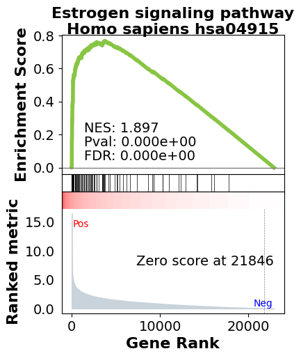
2.12. GSEA enrichment plots
Visualize the running enrichment score with obj.plot() (or the standalone gseaplot / gseaplot2 helpers). Pass ofname='figure.pdf' to save to disk.
[36]:
pre_res.res2d.head(5)
[36]:
| Name | Term | ES | NES | NOM p-val | FDR q-val | FWER p-val | Tag % | Gene % | Lead_genes | |
|---|---|---|---|---|---|---|---|---|---|---|
| 0 | prerank | Adherens junction Homo sapiens hsa04520 | 0.784625 | 1.917092 | 0.0 | 0.0 | 0.0 | 47/74 | 10.37% | CTNNB1;EGFR;RAC1;TGFBR1;SMAD4;MET;EP300;CDC42;... |
| 1 | prerank | Estrogen signaling pathway Homo sapiens hsa04915 | 0.766347 | 1.896928 | 0.0 | 0.0 | 0.0 | 74/99 | 16.57% | CALM1;PRKACA;GRB2;SP1;EGFR;KRAS;HRAS;HSP90AB1;... |
| 2 | prerank | Glioma Homo sapiens hsa05214 | 0.784678 | 1.895572 | 0.0 | 0.0 | 0.0 | 52/65 | 16.29% | CALM1;GRB2;EGFR;PRKCA;KRAS;HRAS;TP53;MAPK1;PRK... |
| 3 | prerank | Thyroid hormone signaling pathway Homo sapiens... | 0.757700 | 1.890973 | 0.0 | 0.0 | 0.0 | 84/118 | 16.29% | CTNNB1;PRKACA;PRKCA;KRAS;NOTCH1;EP300;CREBBP;H... |
| 4 | prerank | Long-term potentiation Homo sapiens hsa04720 | 0.778249 | 1.890416 | 0.0 | 0.0 | 0.0 | 42/66 | 9.01% | CALM1;PRKACA;PRKCA;KRAS;EP300;CREBBP;HRAS;PRKA... |
[37]:
# Plot a single term by name. obj.plot() is the convenient wrapper (v1.0.5+).
terms = pre_res.res2d.Term
axs = pre_res.plot(terms=terms[1])

# For finer control, use the standalone helper:
# from gseapy import gseaplot
# gseaplot(rank_metric=pre_res.ranking, term=terms[0],
#          ofname='your.plot.pdf', **pre_res.results[terms[0]])
Plot several pathways together in one figure.
[38]:
axs = pre_res.plot(
    terms=terms[1:5],
    show_ranking=True,     # show the ranking metric on a secondary y-axis
    figsize=(3, 4),
    # legend_kws={'loc': (1.2, 0)},  # reposition the legend if needed
)

# Equivalent low-level call:
# from gseapy import gseaplot2
# terms = pre_res.res2d.Term[1:5]
# hits  = [pre_res.results[t]['hits'] for t in terms]
# runes = [pre_res.results[t]['RES'] for t in terms]
# fig = gseaplot2(terms=terms, ress=runes, hits=hits,
#                 rank_metric=pre_res.ranking, figsize=(4, 5))
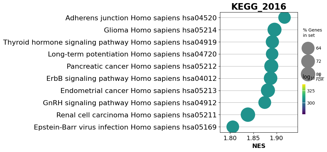
dotplot also works on GSEA results.
[39]:
from gseapy import dotplot

ax = dotplot(
    pre_res.res2d,
    column="FDR q-val",
    title='KEGG_2016',
    cmap=plt.cm.viridis,
    size=6,                # dot size scaling
    figsize=(4, 5),
    cutoff=0.25,           # only show terms with FDR q-val <= cutoff
    show_ring=False,
)
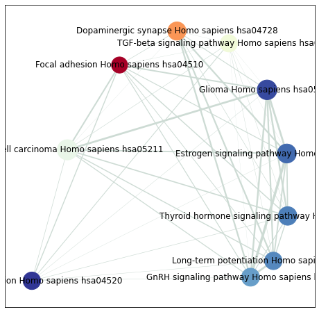
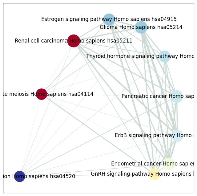
2.13. Network visualization (enrichment map)
enrichment_map builds a network where nodes are enriched terms and edges connect terms that share genes. It returns nodes and edges DataFrames that you can also export for Cytoscape.
[40]:
from gseapy import enrichment_map

# Returns two DataFrames: node table and edge table.
nodes, edges = enrichment_map(pre_res.res2d)
[41]:
import networkx as nx
[42]:
# Build a graph from the edge table; carry similarity coefficients as edge attributes.
G = nx.from_pandas_edgelist(
    edges,
    source='src_idx',
    target='targ_idx',
    edge_attr=['jaccard_coef', 'overlap_coef', 'overlap_genes'],
)
[43]:
fig, ax = plt.subplots(figsize=(8, 8))

# Lay out the nodes.
pos = nx.layout.spiral_layout(G)

# Nodes: color by NES, size by the fraction of genes hit.
nx.draw_networkx_nodes(
    G, pos=pos,
    cmap=plt.cm.RdYlBu,
    node_color=list(nodes.NES),
    node_size=list(nodes.Hits_ratio * 1000),
)
# Node labels (term names).
nx.draw_networkx_labels(G, pos=pos, labels=nodes.Term.to_dict())

# Edges: width proportional to Jaccard similarity.
edge_weight = nx.get_edge_attributes(G, 'jaccard_coef').values()
nx.draw_networkx_edges(
    G, pos=pos,
    width=list(map(lambda x: x * 10, edge_weight)),
    edge_color='#CDDBD4',
)
plt.show()
[44]:
# !gseapy prerank -r temp.rnk -g temp.gmt -o prerank_report_temp
2.13.1. Standard GSEA (gsea)
gp.gsea() runs the classic GSEA on an expression matrix with phenotype labels, computing the ranking metric and a phenotype-permutation null internally.
Accepted inputs
data: aDataFrame(genes × samples), a.gctfile, or a tab-delimited text file.cls: a.clsfile, or a Python list of class labels (one per sample).gene_sets: an Enrichr library name, a.gmtpath, or a{term: [genes]}dict.
Note on symbols: as with
prerank, match your gene identifiers to the library (Enrichr libraries use UPPERCASE human symbols).
[45]:
# A .cls file labels each sample with its phenotype/class.
phenoA, phenoB, class_vector = gp.parser.gsea_cls_parser("./tests/extdata/Leukemia.cls")
[46]:
# class_vector holds the per-sample class label.
print(class_vector)
['ALL', 'ALL', 'ALL', 'ALL', 'ALL', 'ALL', 'ALL', 'ALL', 'ALL', 'ALL', 'ALL', 'ALL', 'ALL', 'ALL', 'ALL', 'ALL', 'ALL', 'ALL', 'ALL', 'ALL', 'ALL', 'ALL', 'ALL', 'ALL', 'AML', 'AML', 'AML', 'AML', 'AML', 'AML', 'AML', 'AML', 'AML', 'AML', 'AML', 'AML', 'AML', 'AML', 'AML', 'AML', 'AML', 'AML', 'AML', 'AML', 'AML', 'AML', 'AML', 'AML']
[47]:
# Expression matrix: genes in rows, samples in columns.
gene_exp = pd.read_csv("./tests/extdata/Leukemia_hgu95av2.trim.txt", sep="\t")
gene_exp.head()
[47]:
| Gene | NAME | ALL_1 | ALL_2 | ALL_3 | ALL_4 | ALL_5 | ALL_6 | ALL_7 | ALL_8 | ... | AML_15 | AML_16 | AML_17 | AML_18 | AML_19 | AML_20 | AML_21 | AML_22 | AML_23 | AML_24 | |
|---|---|---|---|---|---|---|---|---|---|---|---|---|---|---|---|---|---|---|---|---|---|
| 0 | MAPK3 | 1000_at | 1633.6 | 2455.0 | 866.0 | 1000.0 | 3159.0 | 1998.0 | 1580.0 | 1955.0 | ... | 1826.0 | 2849.0 | 2980.0 | 1442.0 | 3672.0 | 294.0 | 2188.0 | 1245.0 | 1934.0 | 13154.0 |
| 1 | TIE1 | 1001_at | 284.4 | 159.0 | 173.0 | 216.0 | 1187.0 | 647.0 | 352.0 | 1224.0 | ... | 1556.0 | 893.0 | 1278.0 | 301.0 | 797.0 | 248.0 | 167.0 | 941.0 | 1398.0 | -502.0 |
| 2 | CYP2C19 | 1002_f_at | 285.8 | 114.0 | 429.0 | -43.0 | 18.0 | 366.0 | 119.0 | -88.0 | ... | -177.0 | 64.0 | -359.0 | 68.0 | 2.0 | -464.0 | -127.0 | -279.0 | 301.0 | 509.0 |
| 3 | CXCR5 | 1003_s_at | -126.6 | -388.0 | 143.0 | -915.0 | -439.0 | -371.0 | -448.0 | -862.0 | ... | 237.0 | -834.0 | -1940.0 | -684.0 | -1236.0 | -1561.0 | -895.0 | -1016.0 | -2238.0 | -1362.0 |
| 4 | CXCR5 | 1004_at | -83.3 | 33.0 | 195.0 | 85.0 | 54.0 | -6.0 | 55.0 | 101.0 | ... | 86.0 | -5.0 | 487.0 | 102.0 | 33.0 | -153.0 | -50.0 | 257.0 | 439.0 | 386.0 |
5 rows × 50 columns
[48]:
print("Positively correlated phenotype:", phenoA)
print("Negatively correlated phenotype:", phenoB)
Positively correlated phenotype: ALL
Negatively correlated phenotype: AML
[49]:
gs_res = gp.gsea(
    data=gene_exp,                                       # or a .gct / .txt path
    gene_sets='./tests/extdata/h.all.v7.0.symbols.gmt',  # or an Enrichr library name
    cls="./tests/extdata/Leukemia.cls",                  # or cls=class_vector
    permutation_type='phenotype',  # use 'phenotype' when each group has >= 15 samples
    permutation_num=1000,          # reduced for the demo
    outdir=None,
    method='signal_to_noise',      # ranking metric
    threads=4,
    seed=7,
)
2026-06-24 11:24:17,956 [WARNING] Found duplicated gene names, values averaged by gene names!
You can also use the GSEA class directly and set the phenotype labels manually via pheno_pos / pheno_neg.
[50]:
from gseapy import GSEA

gs = GSEA(
    data=gene_exp,
    gene_sets='KEGG_2016',
    classes=class_vector,          # or cls=class_vector
    permutation_type='phenotype',
    permutation_num=1000,
    outdir=None,
    method='signal_to_noise',
    threads=4,
    seed=8,
)
gs.pheno_pos = "AML"               # name of the positive phenotype
gs.pheno_neg = "ALL"               # name of the negative phenotype
gs.run()
2026-06-24 11:24:19,582 [WARNING] Found duplicated gene names, values averaged by gene names!
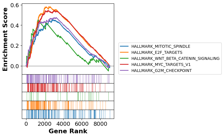
2.14. GSEA plots
The gsea module can auto-generate per-set heatmaps in the background. To plot yourself, use the snippets below.
[51]:
# Running enrichment score for the top 5 terms.
terms = gs_res.res2d.Term
axs = gs_res.plot(terms[:5], show_ranking=False, legend_kws={'loc': (1.05, 0)})
[52]:
# Low-level equivalent with gseaplot2:
# from gseapy import gseaplot2
# terms = gs_res.res2d.Term[:5]
# hits  = [gs_res.results[t]['hits'] for t in terms]
# runes = [gs_res.results[t]['RES'] for t in terms]
# fig = gseaplot2(terms=terms, ress=runes, hits=hits,
#                 rank_metric=gs_res.ranking, figsize=(4, 5))
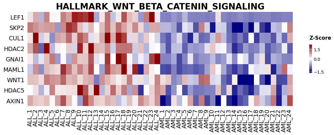
[53]:
from gseapy import heatmap

# Heatmap of the leading-edge genes for one enriched term.
i = 2
genes = gs_res.res2d.Lead_genes[i].split(";")
# z_score=0 standardizes across rows (genes). Pass ofname='figure.pdf' to save.
ax = heatmap(df=gs_res.heatmat.loc[genes], z_score=0, title=terms[i], figsize=(14, 4))
[54]:
# The underlying expression values behind that heatmap.
gs_res.heatmat.loc[genes]
[54]:
| ALL_1 | ALL_2 | ALL_3 | ALL_4 | ALL_5 | ALL_6 | ALL_7 | ALL_8 | ALL_9 | ALL_10 | ... | AML_15 | AML_16 | AML_17 | AML_18 | AML_19 | AML_20 | AML_21 | AML_22 | AML_23 | AML_24 | |
|---|---|---|---|---|---|---|---|---|---|---|---|---|---|---|---|---|---|---|---|---|---|
| Gene | |||||||||||||||||||||
| LEF1 | 8544.10 | 12552.0 | 2869.0 | 15265.0 | 7446.0 | 6991.0 | 15520.0 | 13114.0 | 22604.0 | 21795.0 | ... | 682.0 | 152.0 | -348.0 | 30.0 | 210.0 | 350.0 | -242.0 | -47.0 | 176.0 | 14.0 |
| SKP2 | 23.80 | -45.0 | -95.0 | -71.0 | -65.0 | -547.0 | -24.0 | 230.0 | 159.0 | -162.0 | ... | -865.0 | -642.0 | -1005.0 | -413.0 | -733.0 | -812.0 | -464.0 | -490.0 | -333.0 | 7.0 |
| CUL1 | 1712.75 | 3309.0 | 1273.5 | 1726.5 | 947.5 | 2160.0 | 2065.0 | 2524.5 | 1882.5 | 2684.5 | ... | 851.5 | 614.5 | 1560.0 | 523.0 | 952.0 | 935.0 | 646.0 | 1214.5 | 770.0 | 2088.5 |
| HDAC2 | 4542.90 | 6030.0 | 1195.0 | 9368.0 | 2281.0 | 3407.0 | 3175.0 | 3962.0 | 2616.0 | 6848.0 | ... | 1072.0 | 1918.0 | 1545.0 | 1653.0 | 2328.0 | 1061.0 | 1571.0 | 1749.0 | 2942.0 | 1174.0 |
| GNAI1 | 588.50 | 163.0 | 364.0 | 882.0 | 1317.0 | 17.0 | 518.0 | 89.0 | 1136.0 | 816.0 | ... | 470.0 | 313.0 | -163.0 | 210.0 | 684.0 | -331.0 | 115.0 | 55.0 | -80.0 | -94.0 |
| MAML1 | 871.40 | 1871.0 | 578.0 | 1589.0 | 1448.0 | 1364.0 | 2494.0 | 1989.0 | 1538.0 | 1946.0 | ... | 390.0 | 233.0 | 1075.0 | 962.0 | 997.0 | 1316.0 | 48.0 | 609.0 | 2090.0 | 1056.0 |
| WNT1 | -872.50 | -875.0 | -1012.0 | -535.0 | -654.0 | -694.0 | -421.0 | -827.0 | -770.0 | -1001.0 | ... | -2506.0 | -2791.0 | -2249.0 | -1201.0 | -1819.0 | -2599.0 | -995.0 | -1861.0 | -1835.0 | -714.0 |
| HDAC5 | 2137.20 | 2374.0 | 1651.0 | 2012.0 | 3132.0 | 2279.0 | 2314.0 | 2349.0 | 2376.0 | 5455.0 | ... | 1215.0 | 1024.0 | 760.0 | 1368.0 | 1923.0 | 1927.0 | 2872.0 | 848.0 | 1629.0 | 2763.0 |
| AXIN1 | -433.50 | -722.0 | -808.0 | -623.0 | -1167.0 | -326.0 | 448.0 | -661.0 | -1315.0 | -1991.0 | ... | -2590.0 | -2417.0 | -1321.0 | -466.0 | -1628.0 | -1910.0 | 93.0 | -2951.0 | -1666.0 | 471.0 |
9 rows × 48 columns
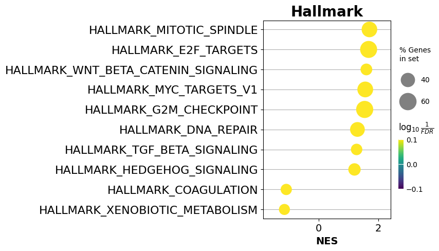
[55]:
from gseapy import dotplot

ax = dotplot(
    gs_res.res2d,
    column="FDR q-val",
    title='Hallmark',
    cmap=plt.cm.viridis,
    size=5,
    figsize=(4, 5),
    cutoff=1,              # show all terms (no significance filter)
)
2.15. Command-line equivalent
[56]:
# !gseapy gsea -d ./tests/extdata/Leukemia_hgu95av2.trim.txt \
#              -g KEGG_2016 -c ./tests/extdata/Leukemia.cls \
#              -o test/gsea_report \
#              -v --no-plot \
#              -t phenotype
2.15.1. Single-sample GSEA (ssgsea)
gp.ssgsea() scores each sample independently, producing an enrichment score per gene set per sample — useful when you do not have two phenotype groups to contrast.
Not sure whether to use prerank or ssgsea? See the FAQ.
Accepted ``data`` inputs: a .txt/.gct file, a DataFrame (genes × samples), or a Series indexed by gene. gene_sets accepts the usual name / .gmt / dict.
[57]:
ss = gp.ssgsea(
    data='./tests/extdata/Leukemia_hgu95av2.trim.txt',
    gene_sets='./tests/extdata/h.all.v7.0.symbols.gmt',
    outdir=None,
    sample_norm_method='rank',   # 'rank' ranks genes per sample; 'custom' uses raw values
    no_plot=True,
)
2026-06-24 11:24:23,205 [WARNING] Found duplicated gene names, values averaged by gene names!
[58]:
ss.res2d.head()
[58]:
| Name | Term | ES | NES | |
|---|---|---|---|---|
| 0 | ALL_2 | HALLMARK_MYC_TARGETS_V1 | 3393.823575 | 0.707975 |
| 1 | ALL_12 | HALLMARK_MYC_TARGETS_V1 | 3385.626111 | 0.706265 |
| 2 | AML_11 | HALLMARK_MYC_TARGETS_V1 | 3359.186716 | 0.700749 |
| 3 | ALL_14 | HALLMARK_MYC_TARGETS_V1 | 3348.938881 | 0.698611 |
| 4 | ALL_17 | HALLMARK_MYC_TARGETS_V1 | 3335.065348 | 0.695717 |
[59]:
# ssGSEA also accepts a DataFrame or Series (gene symbols as the index).
ssdf = pd.read_csv("./tests/data/temp.rnk", header=None, index_col=0, sep="\t")
ssdf.head()
[59]:
| 1 | |
|---|---|
| 0 | |
| ATXN1 | 16.456753 |
| UBQLN4 | 13.989493 |
| CALM1 | 13.745533 |
| DLG4 | 12.796588 |
| MRE11A | 12.787631 |
[60]:
# Collapse the single-column DataFrame to a Series.
ssdf2 = ssdf.squeeze()
[61]:
# Series / DataFrame input is supported directly.
temp = gp.ssgsea(data=ssdf2, gene_sets="./tests/data/temp.gmt")
2.16. Access the enrichment scores (ES / NES)
Results live on obj.res2d. Pivot to a term × sample matrix for downstream use.
[62]:
ss.res2d.sort_values('Name').head()
[62]:
| Name | Term | ES | NES | |
|---|---|---|---|---|
| 601 | ALL_1 | HALLMARK_PANCREAS_BETA_CELLS | -1280.654659 | -0.267153 |
| 934 | ALL_1 | HALLMARK_APOPTOSIS | 970.818772 | 0.202519 |
| 1774 | ALL_1 | HALLMARK_HEDGEHOG_SIGNALING | 431.446694 | 0.090003 |
| 279 | ALL_1 | HALLMARK_INTERFERON_ALPHA_RESPONSE | 1721.458034 | 0.359108 |
| 1778 | ALL_1 | HALLMARK_BILE_ACID_METABOLISM | -429.127871 | -0.089519 |
[63]:
# Reshape to NES values, terms in rows and samples in columns.
nes = ss.res2d.pivot(index='Term', columns='Name', values='NES')
nes.head()
[63]:
| Name | ALL_1 | ALL_10 | ALL_11 | ALL_12 | ALL_13 | ALL_14 | ALL_15 | ALL_16 | ALL_17 | ALL_18 | ... | AML_22 | AML_23 | AML_24 | AML_3 | AML_4 | AML_5 | AML_6 | AML_7 | AML_8 | AML_9 |
|---|---|---|---|---|---|---|---|---|---|---|---|---|---|---|---|---|---|---|---|---|---|
| Term | |||||||||||||||||||||
| HALLMARK_ADIPOGENESIS | 0.287384 | 0.274548 | 0.290059 | 0.285388 | 0.322757 | 0.305239 | 0.275686 | 0.266209 | 0.315803 | 0.282617 | ... | 0.277755 | 0.261477 | 0.200083 | 0.312948 | 0.342963 | 0.253282 | 0.298924 | 0.410395 | 0.387433 | 0.343606 |
| HALLMARK_ALLOGRAFT_REJECTION | 0.061770 | 0.028062 | 0.096589 | 0.080713 | 0.082701 | 0.102735 | 0.125250 | 0.147262 | 0.124621 | 0.091077 | ... | 0.185738 | 0.157852 | 0.055585 | 0.218827 | 0.172395 | 0.199077 | 0.158945 | 0.138350 | 0.110787 | 0.121643 |
| HALLMARK_ANDROGEN_RESPONSE | 0.133453 | 0.113911 | 0.193074 | 0.201531 | 0.151001 | 0.129670 | 0.173563 | 0.144836 | 0.180214 | 0.180801 | ... | 0.180443 | 0.188891 | 0.197979 | 0.174892 | 0.142850 | 0.184843 | 0.157449 | 0.162843 | 0.180475 | 0.181878 |
| HALLMARK_ANGIOGENESIS | -0.113481 | -0.182411 | -0.195637 | -0.094817 | -0.163717 | -0.139243 | -0.119084 | -0.154526 | -0.068290 | -0.121156 | ... | 0.054883 | -0.023782 | 0.119022 | -0.067741 | 0.048430 | 0.012808 | 0.032505 | -0.024058 | -0.039492 | -0.043769 |
| HALLMARK_APICAL_JUNCTION | 0.051372 | 0.063763 | 0.054601 | 0.014385 | 0.049019 | 0.052690 | 0.064787 | 0.052192 | 0.056070 | 0.064936 | ... | 0.109270 | 0.090065 | 0.155801 | 0.091556 | 0.110045 | 0.101659 | 0.128808 | 0.095511 | 0.080076 | 0.098644 |
5 rows × 48 columns
Warning: if you set
permutation_num > 0,ssgseabehaves likeprerankbut with the ssGSEA statistic. Do not do this unless you know exactly why you need it.ss_permut = gp.ssgsea( data="./tests/extdata/Leukemia_hgu95av2.trim.txt", gene_sets="./tests/extdata/h.all.v7.0.symbols.gmt", outdir=None, sample_norm_method='rank', permutation_num=20, # > 0 makes it behave like prerank no_plot=True, threads=4, seed=9, ) ss_permut.res2d.head(5)
2.17. Command-line equivalent
[64]:
# !gseapy ssgsea -d ./tests/extdata/Leukemia_hgu95av2.trim.txt \
#                -g ./tests/data/temp.gmt \
#                -o test/ssgsea_report \
#                -p 4 --no-plot
2.17.1. Gene Set Variation Analysis (gsva)
gp.gsva() is GSEApy’s port of GSVA — an unsupervised method that turns a gene × sample expression matrix into a gene-set × sample matrix of enrichment scores, with no phenotype labels required.
[65]:
es = gp.gsva(
    data='./tests/extdata/Leukemia_hgu95av2.trim.txt',
    gene_sets='./tests/extdata/h.all.v7.0.symbols.gmt',
    outdir=None,
)
2026-06-24 11:24:23,575 [WARNING] Found duplicated gene names, values averaged by gene names!
[66]:
# Reshape to a gene-set x sample matrix of GSVA enrichment scores.
es.res2d.pivot(index='Term', columns='Name', values='ES').head()
[66]:
| Name | ALL_1 | ALL_10 | ALL_11 | ALL_12 | ALL_13 | ALL_14 | ALL_15 | ALL_16 | ALL_17 | ALL_18 | ... | AML_22 | AML_23 | AML_24 | AML_3 | AML_4 | AML_5 | AML_6 | AML_7 | AML_8 | AML_9 |
|---|---|---|---|---|---|---|---|---|---|---|---|---|---|---|---|---|---|---|---|---|---|
| Term | |||||||||||||||||||||
| HALLMARK_ADIPOGENESIS | -0.213310 | -0.080960 | 0.003289 | -0.017909 | 0.207841 | 0.023294 | -0.085392 | -0.221273 | 0.161470 | -0.018250 | ... | 0.033440 | -0.190436 | -0.098500 | 0.105208 | 0.196799 | -0.296305 | -0.084042 | 0.450832 | 0.226921 | 0.209835 |
| HALLMARK_ALLOGRAFT_REJECTION | -0.210468 | -0.373787 | -0.086016 | -0.169623 | -0.158775 | -0.016488 | -0.050703 | 0.104430 | -0.075816 | -0.193654 | ... | 0.023653 | 0.032892 | -0.113577 | 0.307030 | 0.134581 | 0.188905 | 0.132169 | 0.024078 | -0.092054 | -0.195987 |
| HALLMARK_ANDROGEN_RESPONSE | -0.136330 | -0.308572 | 0.008126 | 0.048490 | -0.061181 | -0.203036 | 0.070416 | -0.125240 | 0.080075 | 0.022248 | ... | 0.031898 | 0.064394 | 0.070232 | 0.199349 | -0.079399 | -0.016658 | -0.127327 | 0.018847 | 0.121426 | 0.163149 |
| HALLMARK_ANGIOGENESIS | 0.035895 | -0.287645 | -0.214951 | -0.291145 | -0.311917 | -0.236717 | -0.345662 | -0.250202 | -0.233296 | -0.318353 | ... | 0.244374 | -0.076852 | -0.010928 | -0.210787 | 0.387912 | 0.269447 | 0.348230 | 0.157249 | 0.075479 | -0.064515 |
| HALLMARK_APICAL_JUNCTION | -0.088652 | -0.128757 | -0.050282 | -0.248682 | -0.145164 | 0.001997 | -0.082962 | -0.091691 | -0.168941 | -0.139766 | ... | 0.005859 | -0.067385 | 0.062719 | -0.022434 | 0.076593 | 0.138664 | 0.240647 | 0.039307 | 0.016764 | 0.057512 |
5 rows × 48 columns
2.18. Command-line equivalent
[67]:
# !gseapy gsva -d ./tests/data/expr.gsva.csv \
#              -g ./tests/data/geneset.gsva.gmt \
#              -o test/gsva_report
2.18.1. Replot (replot)
gp.replot() re-creates GSEA plots from the output of the Broad Institute’s Java GSEA application. It needs the edb/ folder produced by that tool, with this layout:
data/
└── edb/
    ├── C1OE.cls
    ├── gene_sets.gmt
    ├── gsea_data.gsea_data.rnk
    └── results.edb
[68]:
rep = gp.replot(indir="./tests/data", outdir="tests/replot_test")
2.19. Command-line equivalent
[69]:
# !gseapy replot -i data -o test/replot_test