2. GSEAPY Example
Examples to use GSEApy inside python console
[1]:
# %matplotlib inline
# %config InlineBackend.figure_format='retina' # mac
%load_ext autoreload
%autoreload 2
import pandas as pd
import gseapy as gp
import matplotlib.pyplot as plt
Check gseapy version
[2]:
gp.__version__
[2]:
'1.1.0'
2.1. Biomart API
Don’t use this if you don’t know Biomart
Warning: This API has limited support now
2.1.1. Convert gene identifiers
[3]:
from gseapy import Biomart
bm = Biomart()
[4]:
## view validated marts
# marts = bm.get_marts()
## view validated dataset
# datasets = bm.get_datasets(mart='ENSEMBL_MART_ENSEMBL')
## view validated attributes
# attrs = bm.get_attributes(dataset='hsapiens_gene_ensembl')
## view validated filters
# filters = bm.get_filters(dataset='hsapiens_gene_ensembl')
## query results
queries ={'ensembl_gene_id': ['ENSG00000125285','ENSG00000182968'] } # need to be a dict object
results = bm.query(dataset='hsapiens_gene_ensembl',
                   attributes=['ensembl_gene_id', 'external_gene_name', 'entrezgene_id', 'go_id'],
                   filters=queries)
results.tail()
[4]:
| ensembl_gene_id | external_gene_name | entrezgene_id | go_id | |
|---|---|---|---|---|
| 36 | ENSG00000182968 | SOX1 | 6656 | GO:0021884 |
| 37 | ENSG00000182968 | SOX1 | 6656 | GO:0030900 |
| 38 | ENSG00000182968 | SOX1 | 6656 | GO:0048713 |
| 39 | ENSG00000182968 | SOX1 | 6656 | GO:1904936 |
| 40 | ENSG00000182968 | SOX1 | 6656 | GO:1990830 |
[5]:
results.dtypes
[5]:
ensembl_gene_id       object
external_gene_name    object
entrezgene_id          Int32
go_id                 object
dtype: object
2.1.2. Mouse gene symbols maps to Human, or Vice Versa
This is useful when you have troubles to convert gene symbols between human and mouse
[6]:
from gseapy import Biomart
bm = Biomart()
# note the dataset and attribute names are different
m2h = bm.query(dataset='mmusculus_gene_ensembl',
               attributes=['ensembl_gene_id','external_gene_name',
                           'hsapiens_homolog_ensembl_gene',
                           'hsapiens_homolog_associated_gene_name'])

h2m = bm.query(dataset='hsapiens_gene_ensembl',
               attributes=['ensembl_gene_id','external_gene_name',
                           'mmusculus_homolog_ensembl_gene',
                           'mmusculus_homolog_associated_gene_name'])
[7]:
# h2m.sample(10)
2.1.3. Gene Symbols Conversion for the GMT file
This is useful when runing GSEA for non-human species
e.g. Convert Human gene symbols to Mouse.
[8]:
# get a dict symbol mappings
h2m_dict = {}
for i, row in h2m.loc[:,["external_gene_name", "mmusculus_homolog_associated_gene_name"]].iterrows():
    if row.isna().any(): continue
    h2m_dict[row['external_gene_name']] = row["mmusculus_homolog_associated_gene_name"]
# read gmt file into dict
kegg = gp.read_gmt(path="tests/extdata/enrichr.KEGG_2016.gmt")
print(kegg['MAPK signaling pathway Homo sapiens hsa04010'][:10])
['EGF', 'IL1R1', 'IL1R2', 'HSPA1L', 'CACNA2D2', 'CACNA2D1', 'CACNA2D4', 'CACNA2D3', 'MAPK8IP3', 'MAPK8IP1']
[9]:
kegg_mouse = {}
for term, genes in kegg.items():
    new_genes = []
    for gene in genes:
        if gene in h2m_dict:
            new_genes.append(h2m_dict[gene])
    kegg_mouse[term] = new_genes
print(kegg_mouse['MAPK signaling pathway Homo sapiens hsa04010'][:10])
['Egf', 'Il1r1', 'Il1r2', 'Hspa1l', 'Cacna2d2', 'Cacna2d1', 'Cacna2d4', 'Cacna2d3', 'Mapk8ip3', 'Mapk8ip1']
2.2. Msigdb API
Down load gmt file from: https://data.broadinstitute.org/gsea-msigdb/msigdb/release/
[10]:
from gseapy import Msigdb
[11]:
msig = Msigdb()
# mouse hallmark gene sets
gmt = msig.get_gmt(category='mh.all', dbver="2023.1.Mm")
two helper method
# list msigdb version you wanna query
msig.list_dbver()
# list categories given dbver.
msig.list_category(dbver="2023.1.Hs") # mouse
[12]:
print(gmt['HALLMARK_WNT_BETA_CATENIN_SIGNALING'])
['Ctnnb1', 'Jag1', 'Myc', 'Notch1', 'Ptch1', 'Trp53', 'Axin1', 'Ncstn', 'Rbpj', 'Psen2', 'Wnt1', 'Axin2', 'Hey2', 'Fzd1', 'Frat1', 'Csnk1e', 'Dvl2', 'Hey1', 'Gnai1', 'Lef1', 'Notch4', 'Ppard', 'Adam17', 'Tcf7', 'Numb', 'Ccnd2', 'Ncor2', 'Kat2a', 'Nkd1', 'Hdac2', 'Dkk1', 'Wnt5b', 'Wnt6', 'Dll1', 'Skp2', 'Hdac5', 'Fzd8', 'Dkk4', 'Cul1', 'Jag2', 'Hdac11', 'Maml1']
2.3. Enrichr API
See all supported enrichr library names
Select database from { ‘Human’, ‘Mouse’, ‘Yeast’, ‘Fly’, ‘Fish’, ‘Worm’ }
[13]:
# default: Human
names = gp.get_library_name()
names[:10]
[13]:
['ARCHS4_Cell-lines',
 'ARCHS4_IDG_Coexp',
 'ARCHS4_Kinases_Coexp',
 'ARCHS4_TFs_Coexp',
 'ARCHS4_Tissues',
 'Achilles_fitness_decrease',
 'Achilles_fitness_increase',
 'Aging_Perturbations_from_GEO_down',
 'Aging_Perturbations_from_GEO_up',
 'Allen_Brain_Atlas_10x_scRNA_2021']
[14]:
# yeast
yeast = gp.get_library_name(organism='Yeast')
yeast[:10]
[14]:
['Cellular_Component_AutoRIF',
 'Cellular_Component_AutoRIF_Predicted_zscore',
 'GO_Biological_Process_2018',
 'GO_Biological_Process_AutoRIF',
 'GO_Biological_Process_AutoRIF_Predicted_zscore',
 'GO_Cellular_Component_2018',
 'GO_Cellular_Component_AutoRIF',
 'GO_Cellular_Component_AutoRIF_Predicted_zscore',
 'GO_Molecular_Function_2018',
 'GO_Molecular_Function_AutoRIF']
Parse Enrichr library into dict
[15]:
## download library or read a .gmt file
go_mf = gp.get_library(name='GO_Molecular_Function_2018', organism='Yeast')
print(go_mf['ATP binding (GO:0005524)'])
['MLH1', 'ECM10', 'RLI1', 'SSB1', 'SSB2', 'YTA12', 'MSH2', 'CDC6', 'HMI1', 'YNL247W', 'MSH6', 'SSQ1', 'MCM7', 'SRS2', 'HSP104', 'SSA1', 'MCX1', 'SSC1', 'ARP2', 'ARP3', 'SSE1', 'SMC2', 'SSZ1', 'TDA10', 'ORC5', 'VPS4', 'RBK1', 'SSA4', 'NEW1', 'ORC1', 'SSA2', 'KAR2', 'SSA3', 'DYN1', 'PGK1', 'VPS33', 'LHS1', 'CDC123', 'PMS1']
2.3.1. Over-representation analysis by Enrichr web services
The only requirement of input is a list of gene symbols.
For online web services, gene symbols are not case sensitive.
gene_listacceptspd.Seriespd.DataFramelistobjecttxtfile (one gene symbol per row)
gene_setsaccepts:Multi-libraries names supported, separate each name by comma or input a list.
For example:
# gene_list
gene_list="./data/gene_list.txt",
gene_list=glist
# gene_sets
gene_sets='KEGG_2016'
gene_sets='KEGG_2016,KEGG_2013'
gene_sets=['KEGG_2016','KEGG_2013']
[16]:
# read in an example gene list
gene_list = pd.read_csv("./tests/data/gene_list.txt",header=None, sep="\t")
gene_list.head()
[16]:
| 0 | |
|---|---|
| 0 | IGKV4-1 |
| 1 | CD55 |
| 2 | IGKC |
| 3 | PPFIBP1 |
| 4 | ABHD4 |
[17]:
# convert dataframe or series to list
glist = gene_list.squeeze().str.strip().to_list()
print(glist[:10])
['IGKV4-1', 'CD55', 'IGKC', 'PPFIBP1', 'ABHD4', 'PCSK6', 'PGD', 'ARHGDIB', 'ITGB2', 'CARD6']
2.3.2. Over-representation analysis via Enrichr web services
This is an Example of the Enrichr analysis
NOTE: 1. Enrichr Web Sevices need gene symbols as input 2. Gene symbols will convert to upcases automatically. 3. (Optional) Input an user defined background gene list
2.3.2.1. Enrichr Web Serives (without a backgound input)
[18]:
# if you are only intrested in dataframe that enrichr returned, please set outdir=None
enr = gp.enrichr(gene_list=gene_list, # or "./tests/data/gene_list.txt",
                 gene_sets=['MSigDB_Hallmark_2020','KEGG_2021_Human'],
                 organism='human', # don't forget to set organism to the one you desired! e.g. Yeast
                 outdir=None, # don't write to disk
                )
[19]:
# obj.results stores all results
enr.results.head(5)
[19]:
| Gene_set | Term | Overlap | P-value | Adjusted P-value | Old P-value | Old Adjusted P-value | Odds Ratio | Combined Score | Genes | |
|---|---|---|---|---|---|---|---|---|---|---|
| 0 | MSigDB_Hallmark_2020 | IL-6/JAK/STAT3 Signaling | 19/87 | 1.197225e-09 | 5.986123e-08 | 0 | 0 | 6.844694 | 140.612324 | IL4R;TGFB1;IL1R1;IFNGR1;IL10RB;ITGB3;IFNGR2;IL... |
| 1 | MSigDB_Hallmark_2020 | TNF-alpha Signaling via NF-kB | 27/200 | 3.220898e-08 | 5.368163e-07 | 0 | 0 | 3.841568 | 66.270963 | BTG2;BCL2A1;PLEK;IRS2;LITAF;IFIH1;PANX1;DRAM1;... |
| 2 | MSigDB_Hallmark_2020 | Complement | 27/200 | 3.220898e-08 | 5.368163e-07 | 0 | 0 | 3.841568 | 66.270963 | FCN1;LRP1;PLEK;LIPA;CA2;CASP3;LAMP2;S100A12;FY... |
| 3 | MSigDB_Hallmark_2020 | Inflammatory Response | 24/200 | 1.635890e-06 | 2.044862e-05 | 0 | 0 | 3.343018 | 44.540108 | LYN;IFITM1;BTG2;IL4R;CD82;IL1R1;IFNGR2;ITGB3;F... |
| 4 | MSigDB_Hallmark_2020 | heme Metabolism | 23/200 | 5.533816e-06 | 5.533816e-05 | 0 | 0 | 3.181358 | 38.509172 | SLC22A4;MPP1;BNIP3L;BTG2;ARHGEF12;NEK7;GDE1;FO... |
2.3.2.2. Enrichr Web Service (with backround input)
NOTE: Missing Overlap column in final output
[20]:
# backgound only reconigized a gene list input.
enr_bg = gp.enrichr(gene_list=gene_list,
                 gene_sets=['MSigDB_Hallmark_2020','KEGG_2021_Human'],
                 # organism='human', # organism argment is ignored because user input a background
                 background="tests/data/background.txt",
                 outdir=None, # don't write to disk
                )
[21]:
enr_bg.results.head() #
[21]:
| Gene_set | Term | P-value | Adjusted P-value | Old P-value | Old adjusted P-value | Odds Ratio | Combined Score | Genes | |
|---|---|---|---|---|---|---|---|---|---|
| 0 | MSigDB_Hallmark_2020 | IL-6/JAK/STAT3 Signaling | 3.559435e-11 | 1.779718e-09 | 0 | 0 | 8.533251 | 205.300064 | IL4R;TGFB1;IL1R1;IFNGR1;IL10RB;ITGB3;IFNGR2;IL... |
| 1 | MSigDB_Hallmark_2020 | TNF-alpha Signaling via NF-kB | 3.401526e-10 | 6.356588e-09 | 0 | 0 | 4.824842 | 105.189414 | BTG2;BCL2A1;PLEK;IRS2;LITAF;IFIH1;PANX1;DRAM1;... |
| 2 | MSigDB_Hallmark_2020 | Complement | 3.813953e-10 | 6.356588e-09 | 0 | 0 | 4.796735 | 104.027683 | FCN1;LRP1;PLEK;LIPA;CA2;CASP3;LAMP2;S100A12;FY... |
| 3 | MSigDB_Hallmark_2020 | Inflammatory Response | 3.380686e-08 | 4.225857e-07 | 0 | 0 | 4.197067 | 72.200480 | LYN;IFITM1;BTG2;IL4R;CD82;IL1R1;IFNGR2;ITGB3;F... |
| 4 | MSigDB_Hallmark_2020 | heme Metabolism | 8.943634e-08 | 8.943634e-07 | 0 | 0 | 4.111306 | 66.725423 | SLC22A4;MPP1;BNIP3L;BTG2;ARHGEF12;NEK7;GDE1;FO... |
2.3.3. Over-representation analysis (hypergeometric test) by offline
This API DO NOT use Enrichr web services.
NOTE: 1. The input gene symbols are case sensitive. 2. You need to match the type of the gene identifers which used in your gene_list input and GMT file. 3. Input a .gmt file or gene_set dict object for the argument gene_sets
For example:
gene_sets="./data/genes.gmt",
gene_sets={'A':['gene1', 'gene2',...],
           'B':['gene2', 'gene4',...],
           ...}
[22]:
# NOTE: `enrich` instead of `enrichr`
enr2 = gp.enrich(gene_list="./tests/data/gene_list.txt", # or gene_list=glist
                 gene_sets=["./tests/data/genes.gmt", "unknown", kegg ], # kegg is a dict object
                 background=None, # or "hsapiens_gene_ensembl", or int, or text file, or a list of genes
                 outdir=None,
                 verbose=True)
2023-10-25 10:46:28,796 [INFO] User defined gene sets is given: ./tests/data/genes.gmt
2023-10-25 10:46:28,813 [INFO] Input dict object named with gs_ind_2
2023-10-25 10:46:29,289 [WARNING] Input library not found: unknown. Skip
2023-10-25 10:46:29,291 [INFO] Run: genes.gmt
2023-10-25 10:46:29,293 [INFO] Background is not set! Use all 682 genes in genes.gmt.
2023-10-25 10:46:29,302 [INFO] Run: gs_ind_2
2023-10-25 10:46:29,327 [INFO] Done.
[23]:
enr2.results.head()
[23]:
| Gene_set | Term | Overlap | P-value | Adjusted P-value | Odds Ratio | Combined Score | Genes | |
|---|---|---|---|---|---|---|---|---|
| 0 | genes.gmt | BvA_UpIN_A | 8/139 | 0.457390 | 0.568432 | 1.161982 | 0.908925 | PCSK6;MAP3K5;MBOAT2;MSRB2;IQGAP2;HAL;PADI2;IL1R1 |
| 1 | genes.gmt | BvA_UpIN_B | 12/130 | 0.026744 | 0.187208 | 2.160059 | 7.822534 | FAM65B;MBNL3;GPX8;DYSF;KCTD12;HEBP1;SUOX;ARHGD... |
| 2 | genes.gmt | CvA_UpIN_A | 1/12 | 0.481190 | 0.568432 | 2.266479 | 1.657913 | MBOAT2 |
| 3 | genes.gmt | DvA_UpIN_A | 16/284 | 0.426669 | 0.568432 | 1.127395 | 0.960255 | PCSK6;FXYD6;IFNGR2;MAP3K5;MBOAT2;VNN1;IQGAP2;H... |
| 4 | genes.gmt | DvA_UpIN_D | 13/236 | 0.487227 | 0.568432 | 1.084567 | 0.779830 | GNB4;FAM198B;FAM65B;TXNDC5;GLIPR2;MBNL3;GPX8;D... |
2.3.3.1. About Background genes
By default, all genes in the gene_sets input will be used as background.
However, a better background genes would be the following:
(Recommended) Input a list of background genes: [‘gene1’, ‘gene2’,…]
The background gene list is defined by your experment. e.g. the expressed genes in your RNA-seq.
The gene identifer in gmt/dict should be the same type to the backgound genes.
Specify a number: e.g. 20000. (the number of total expressed genes).
This works, but not recommend. It assumes that all your genes could be found in background.
If genes exist in gmt but not included in background provided, they will affect the significance of the statistical test.
Set a Biomart dataset name: e.g. “hsapiens_gene_ensembl”
The background will use all annotated genes from the
BioMart datasetsyou’ve choosen.The program will try to retrieve the background information automatically.
2.3.4. Plotting
Show top 5 terms of each gene_set ranked by “Adjusted P-value”
[24]:
# simple plotting function
from gseapy import barplot, dotplot
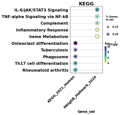
[25]:
# categorical scatterplot
ax = dotplot(enr.results,
              column="Adjusted P-value",
              x='Gene_set', # set x axis, so you could do a multi-sample/library comparsion
              size=10,
              top_term=5,
              figsize=(3,5),
              title = "KEGG",
              xticklabels_rot=45, # rotate xtick labels
              show_ring=True, # set to False to revmove outer ring
              marker='o',
             )
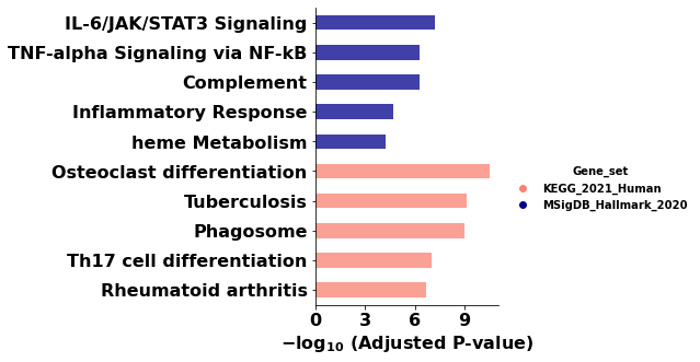
[26]:
# categorical scatterplot
ax = barplot(enr.results,
              column="Adjusted P-value",
              group='Gene_set', # set group, so you could do a multi-sample/library comparsion
              size=10,
              top_term=5,
              figsize=(3,5),
              #color=['darkred', 'darkblue'] # set colors for group
              color = {'KEGG_2021_Human': 'salmon', 'MSigDB_Hallmark_2020':'darkblue'}
             )
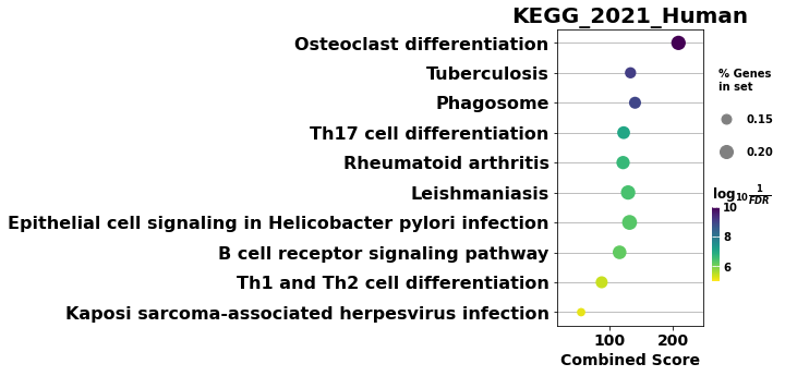
[27]:
# to save your figure, make sure that ``ofname`` is not None
ax = dotplot(enr.res2d, title='KEGG_2021_Human',cmap='viridis_r', size=10, figsize=(3,5))
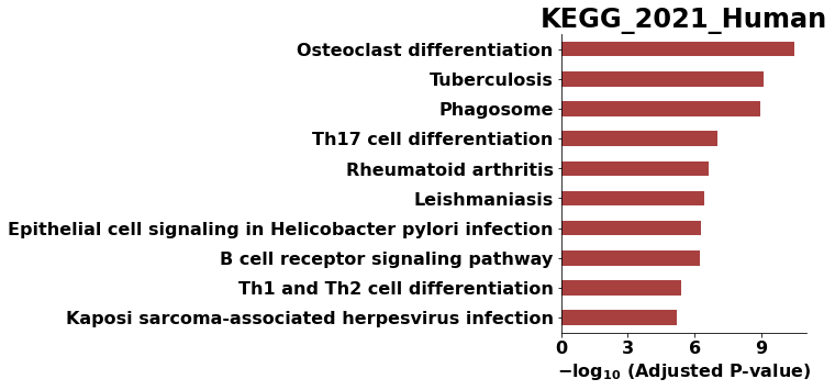
[28]:
# to save your figure, make sure that ``ofname`` is not None
ax = barplot(enr.res2d,title='KEGG_2021_Human', figsize=(4, 5), color='darkred')
2.3.5. Command line usage
the option -v will print out the progress of your job
[29]:
# !gseapy enrichr -i ./data/gene_list.txt \
#                 -g GO_Biological_Process_2017 \
#                 -v -o test/enrichr_BP
2.4. Prerank example
2.4.1. Assign prerank() with
pd.DataFrame: Only contains two columns, or one cloumn with gene_name indexed
pd.Series
a txt file:
GSEApy will skip any data after “#”.
Do not include header in your gene list !
2.4.1.1. NOTE: UPCASES for gene symbols by Default
Gene symbols are all “UPCASES” in the Enrichr Libaries. You should convert your input gene identifier to “UPCASES” first.
If input
gmt,dictobject, please refer to1.2 Mouse gene symbols maps to Human, or Vice Versa(in this page) to convert gene identifier
2.4.1.2. Supported gene_sets input
For example:
gene_sets="KEGG_2016",
gene_sets="KEGG_2016,KEGG2013",
gene_sets="./data/genes.gmt",
gene_sets=["KEGG_2016","./data/genes.gmt"],
gene_sets={'A':['gene1', 'gene2',...],
           'B':['gene2', 'gene4',...],
           ...}
[30]:
rnk = pd.read_csv("./tests/data/temp.rnk", header=None, index_col=0, sep="\t")
rnk.head()
[30]:
| 1 | |
|---|---|
| 0 | |
| ATXN1 | 16.456753 |
| UBQLN4 | 13.989493 |
| CALM1 | 13.745533 |
| DLG4 | 12.796588 |
| MRE11A | 12.787631 |
[31]:
rnk.shape
[31]:
(22922, 1)
[32]:
# # run prerank
# # enrichr libraries are supported by prerank module. Just provide the name
# # use 4 process to acceralate the permutation speed
pre_res = gp.prerank(rnk="./tests/data/temp.rnk", # or rnk = rnk,
                     gene_sets='KEGG_2016',
                     threads=4,
                     min_size=5,
                     max_size=1000,
                     permutation_num=1000, # reduce number to speed up testing
                     outdir=None, # don't write to disk
                     seed=6,
                     verbose=True, # see what's going on behind the scenes
                    )
2023-10-25 10:46:30,863 [WARNING] Duplicated values found in preranked stats: 4.97% of genes
The order of those genes will be arbitrary, which may produce unexpected results.
2023-10-25 10:46:30,864 [INFO] Parsing data files for GSEA.............................
2023-10-25 10:46:30,865 [INFO] Enrichr library gene sets already downloaded in: /home/fangzq/.cache/gseapy, use local file
2023-10-25 10:46:30,902 [INFO] 0001 gene_sets have been filtered out when max_size=1000 and min_size=5
2023-10-25 10:46:30,903 [INFO] 0292 gene_sets used for further statistical testing.....
2023-10-25 10:46:30,903 [INFO] Start to run GSEA...Might take a while..................
2023-10-25 10:46:43,563 [INFO] Congratulations. GSEApy runs successfully................
[ ]:
2.4.2. How to generate your GSEA plot inside python console
Visualize it using gseaplot
Make sure that ofname is not None, if you want to save your figure to the disk
[33]:
pre_res.res2d.head(5)
[33]:
| Name | Term | ES | NES | NOM p-val | FDR q-val | FWER p-val | Tag % | Gene % | Lead_genes | |
|---|---|---|---|---|---|---|---|---|---|---|
| 0 | prerank | Adherens junction Homo sapiens hsa04520 | 0.784625 | 1.912548 | 0.0 | 0.0 | 0.0 | 47/74 | 10.37% | CTNNB1;EGFR;RAC1;TGFBR1;SMAD4;MET;EP300;CDC42;... |
| 1 | prerank | Glioma Homo sapiens hsa05214 | 0.784678 | 1.906706 | 0.0 | 0.0 | 0.0 | 52/65 | 16.29% | CALM1;GRB2;EGFR;PRKCA;KRAS;HRAS;TP53;MAPK1;PRK... |
| 2 | prerank | Estrogen signaling pathway Homo sapiens hsa04915 | 0.766347 | 1.897957 | 0.0 | 0.0 | 0.0 | 74/99 | 16.57% | CALM1;PRKACA;GRB2;SP1;EGFR;KRAS;HRAS;HSP90AB1;... |
| 3 | prerank | Thyroid hormone signaling pathway Homo sapiens... | 0.7577 | 1.891815 | 0.0 | 0.0 | 0.0 | 84/118 | 16.29% | CTNNB1;PRKACA;PRKCA;KRAS;NOTCH1;EP300;CREBBP;H... |
| 4 | prerank | Long-term potentiation Homo sapiens hsa04720 | 0.778249 | 1.888739 | 0.0 | 0.0 | 0.0 | 42/66 | 9.01% | CALM1;PRKACA;PRKCA;KRAS;EP300;CREBBP;HRAS;PRKA... |
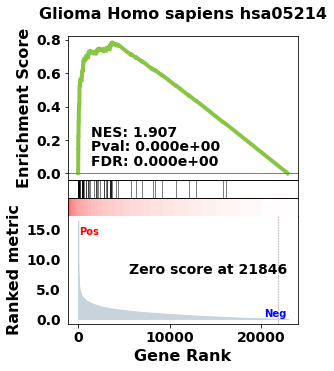
[34]:
## easy way
terms = pre_res.res2d.Term
axs = pre_res.plot(terms=terms[1]) # v1.0.5
# to make more control on the plot, use
# from gseapy import gseaplot
# gseaplot(rank_metric=pre_res.ranking, term=terms[0], ofname='your.plot.pdf', **pre_res.results[terms[0]])
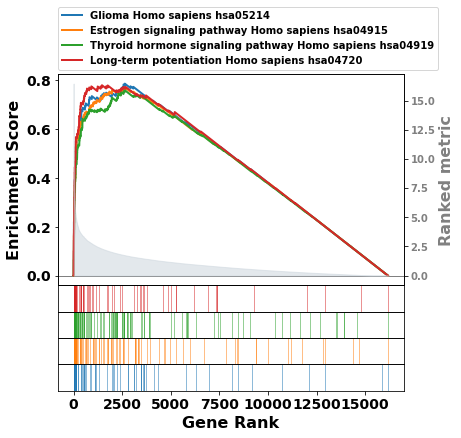
or multi pathway in one
[35]:
axs = pre_res.plot(terms=terms[1:5],
                   #legend_kws={'loc': (1.2, 0)}, # set the legend loc
                   show_ranking=True, # whether to show the second yaxis
                   figsize=(3,4)
                  )
# or use this to have more control on the plot
# from gseapy import gseaplot2
# terms = pre_res.res2d.Term[1:5]
# hits = [pre_res.results[t]['hits'] for t in terms]
# runes = [pre_res.results[t]['RES'] for t in terms]
# fig = gseaplot2(terms=terms, ress=runes, hits=hits,
#               rank_metric=gs_res.ranking,
#               legend_kws={'loc': (1.2, 0)}, # set the legend loc
#               figsize=(4,5)) # rank_metric=pre_res.ranking
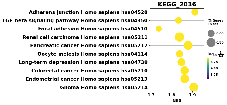
dotplot for GSEA resutls
[36]:
from gseapy import dotplot
# to save your figure, make sure that ``ofname`` is not None
ax = dotplot(pre_res.res2d,
             column="FDR q-val",
             title='KEGG_2016',
             cmap=plt.cm.viridis,
             size=6, # adjust dot size
             figsize=(4,5), cutoff=0.25, show_ring=False)
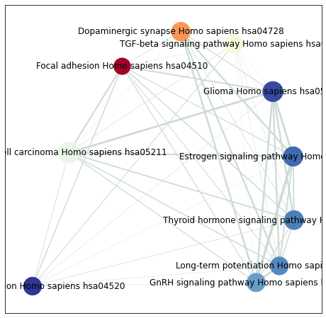
Network Visualization
use
enrichment_mapto build networksave the
nodesandedges. They could be used forcytoscapevisualization.
[37]:
from gseapy import enrichment_map
# return two dataframe
nodes, edges = enrichment_map(pre_res.res2d)
[38]:
import networkx as nx
[39]:
# build graph
G = nx.from_pandas_edgelist(edges,
                            source='src_idx',
                            target='targ_idx',
                            edge_attr=['jaccard_coef', 'overlap_coef', 'overlap_genes'])
[40]:
fig, ax = plt.subplots(figsize=(8, 8))

# init node cooridnates
pos=nx.layout.spiral_layout(G)
#node_size = nx.get_node_attributes()
# draw node
nx.draw_networkx_nodes(G,
                       pos=pos,
                       cmap=plt.cm.RdYlBu,
                       node_color=list(nodes.NES),
                       node_size=list(nodes.Hits_ratio *1000))
# draw node label
nx.draw_networkx_labels(G,
                        pos=pos,
                        labels=nodes.Term.to_dict())
# draw edge
edge_weight = nx.get_edge_attributes(G, 'jaccard_coef').values()
nx.draw_networkx_edges(G,
                       pos=pos,
                       width=list(map(lambda x: x*10, edge_weight)),
                       edge_color='#CDDBD4')
plt.show()
2.4.3. Command line usage
You may also want to use prerank in command line
[41]:
# !gseapy prerank -r temp.rnk -g temp.gmt -o prerank_report_temp
2.5. GSEA Example
2.5.1. Inputs
Assign gsea()
data with:
pandas DataFrame
.gct format file, or a text file
cls with:
a list
a .cls format file
gene_sets with:
gene_sets="KEGG_2016",
gene_sets="KEGG_2016,KEGG2013",
gene_sets="./data/genes.gmt",
gene_sets=["KEGG_2016","./data/genes.gmt"],
gene_sets={'A':['gene1', 'gene2',...],
           'B':['gene2', 'gene4',...],
           ...}
2.5.1.1. NOTE: UPCASES for gene symbols by Default
Gene symbols are all “UPCASES” in the Enrichr Libaries. You should convert your input gene identifier to “UPCASES” first.
If input
gmt,dictobject, please refer to1.2 Mouse gene symbols maps to Human, or Vice Versa(in this page) to convert gene identifier
[42]:
import gseapy as gp
phenoA, phenoB, class_vector =  gp.parser.gsea_cls_parser("./tests/extdata/Leukemia.cls")
[43]:
#class_vector used to indicate group attributes for each sample
print(class_vector)
['ALL', 'ALL', 'ALL', 'ALL', 'ALL', 'ALL', 'ALL', 'ALL', 'ALL', 'ALL', 'ALL', 'ALL', 'ALL', 'ALL', 'ALL', 'ALL', 'ALL', 'ALL', 'ALL', 'ALL', 'ALL', 'ALL', 'ALL', 'ALL', 'AML', 'AML', 'AML', 'AML', 'AML', 'AML', 'AML', 'AML', 'AML', 'AML', 'AML', 'AML', 'AML', 'AML', 'AML', 'AML', 'AML', 'AML', 'AML', 'AML', 'AML', 'AML', 'AML', 'AML']
[44]:
gene_exp = pd.read_csv("./tests/extdata/Leukemia_hgu95av2.trim.txt", sep="\t")
gene_exp.head()
[44]:
| Gene | NAME | ALL_1 | ALL_2 | ALL_3 | ALL_4 | ALL_5 | ALL_6 | ALL_7 | ALL_8 | ... | AML_15 | AML_16 | AML_17 | AML_18 | AML_19 | AML_20 | AML_21 | AML_22 | AML_23 | AML_24 | |
|---|---|---|---|---|---|---|---|---|---|---|---|---|---|---|---|---|---|---|---|---|---|
| 0 | MAPK3 | 1000_at | 1633.6 | 2455.0 | 866.0 | 1000.0 | 3159.0 | 1998.0 | 1580.0 | 1955.0 | ... | 1826.0 | 2849.0 | 2980.0 | 1442.0 | 3672.0 | 294.0 | 2188.0 | 1245.0 | 1934.0 | 13154.0 |
| 1 | TIE1 | 1001_at | 284.4 | 159.0 | 173.0 | 216.0 | 1187.0 | 647.0 | 352.0 | 1224.0 | ... | 1556.0 | 893.0 | 1278.0 | 301.0 | 797.0 | 248.0 | 167.0 | 941.0 | 1398.0 | -502.0 |
| 2 | CYP2C19 | 1002_f_at | 285.8 | 114.0 | 429.0 | -43.0 | 18.0 | 366.0 | 119.0 | -88.0 | ... | -177.0 | 64.0 | -359.0 | 68.0 | 2.0 | -464.0 | -127.0 | -279.0 | 301.0 | 509.0 |
| 3 | CXCR5 | 1003_s_at | -126.6 | -388.0 | 143.0 | -915.0 | -439.0 | -371.0 | -448.0 | -862.0 | ... | 237.0 | -834.0 | -1940.0 | -684.0 | -1236.0 | -1561.0 | -895.0 | -1016.0 | -2238.0 | -1362.0 |
| 4 | CXCR5 | 1004_at | -83.3 | 33.0 | 195.0 | 85.0 | 54.0 | -6.0 | 55.0 | 101.0 | ... | 86.0 | -5.0 | 487.0 | 102.0 | 33.0 | -153.0 | -50.0 | 257.0 | 439.0 | 386.0 |
5 rows × 50 columns
[45]:
print("positively correlated: ", phenoA)
positively correlated: ALL
[46]:
print("negtively correlated: ", phenoB)
negtively correlated: AML
[47]:
# run gsea
# enrichr libraries are supported by gsea module. Just provide the name
gs_res = gp.gsea(data=gene_exp, # or data='./P53_resampling_data.txt'
                 gene_sets='./tests/extdata/h.all.v7.0.symbols.gmt', # or enrichr library names
                 cls= "./tests/extdata/Leukemia.cls", # cls=class_vector
                 # set permutation_type to phenotype if samples >=15
                 permutation_type='phenotype',
                 permutation_num=1000, # reduce number to speed up test
                 outdir=None,  # do not write output to disk
                 method='signal_to_noise',
                 threads=4, seed= 7)
2023-10-25 10:46:47,125 [WARNING] Found duplicated gene names, values averaged by gene names!
You can set pheno_pos, and pheno_neg mannually
[48]:
# example
from gseapy import GSEA
gs = GSEA(data=gene_exp,
         gene_sets='KEGG_2016',
         classes = class_vector, # cls=class_vector
         # set permutation_type to phenotype if samples >=15
         permutation_type='phenotype',
         permutation_num=1000, # reduce number to speed up test
         outdir=None,
         method='signal_to_noise',
         threads=4, seed= 8)
gs.pheno_pos = "AML"
gs.pheno_neg = "ALL"
gs.run()
2023-10-25 10:46:50,381 [WARNING] Found duplicated gene names, values averaged by gene names!
2.5.2. Show the gsea plots
[49]:
terms = gs_res.res2d.Term
axs = gs_res.plot(terms[:5], show_ranking=False, legend_kws={'loc': (1.05, 0)}, )

[50]:
# or use
# from gseapy import gseaplot2

# # multi in one
# terms = gs_res.res2d.Term[:5]
# hits = [gs_res.results[t]['hits'] for t in terms]
# runes = [gs_res.results[t]['RES'] for t in terms]
# fig = gseaplot2(terms=terms, ress=runes, hits=hits,
#               rank_metric=gs_res.ranking,
#               legend_kws={'loc': (1.2, 0)}, # set the legend loc
#               figsize=(4,5)) # rank_metric=pre_res.ranking
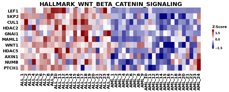
[51]:
from gseapy import heatmap
# plotting heatmap
i = 2
genes = gs_res.res2d.Lead_genes[i].split(";")
# Make sure that ``ofname`` is not None, if you want to save your figure to disk
ax = heatmap(df = gs_res.heatmat.loc[genes], z_score=0, title=terms[i], figsize=(14,4))
[52]:
gs_res.heatmat.loc[genes]
[52]:
| ALL_1 | ALL_2 | ALL_3 | ALL_4 | ALL_5 | ALL_6 | ALL_7 | ALL_8 | ALL_9 | ALL_10 | ... | AML_15 | AML_16 | AML_17 | AML_18 | AML_19 | AML_20 | AML_21 | AML_22 | AML_23 | AML_24 | |
|---|---|---|---|---|---|---|---|---|---|---|---|---|---|---|---|---|---|---|---|---|---|
| Gene | |||||||||||||||||||||
| LEF1 | 8544.10 | 12552.0 | 2869.0 | 15265.0 | 7446.0 | 6991.0 | 15520.0 | 13114.0 | 22604.0 | 21795.0 | ... | 682.0 | 152.0 | -348.0 | 30.0 | 210.0 | 350.0 | -242.0 | -47.0 | 176.0 | 14.0 |
| SKP2 | 23.80 | -45.0 | -95.0 | -71.0 | -65.0 | -547.0 | -24.0 | 230.0 | 159.0 | -162.0 | ... | -865.0 | -642.0 | -1005.0 | -413.0 | -733.0 | -812.0 | -464.0 | -490.0 | -333.0 | 7.0 |
| CUL1 | 1712.75 | 3309.0 | 1273.5 | 1726.5 | 947.5 | 2160.0 | 2065.0 | 2524.5 | 1882.5 | 2684.5 | ... | 851.5 | 614.5 | 1560.0 | 523.0 | 952.0 | 935.0 | 646.0 | 1214.5 | 770.0 | 2088.5 |
| HDAC2 | 4542.90 | 6030.0 | 1195.0 | 9368.0 | 2281.0 | 3407.0 | 3175.0 | 3962.0 | 2616.0 | 6848.0 | ... | 1072.0 | 1918.0 | 1545.0 | 1653.0 | 2328.0 | 1061.0 | 1571.0 | 1749.0 | 2942.0 | 1174.0 |
| GNAI1 | 588.50 | 163.0 | 364.0 | 882.0 | 1317.0 | 17.0 | 518.0 | 89.0 | 1136.0 | 816.0 | ... | 470.0 | 313.0 | -163.0 | 210.0 | 684.0 | -331.0 | 115.0 | 55.0 | -80.0 | -94.0 |
| MAML1 | 871.40 | 1871.0 | 578.0 | 1589.0 | 1448.0 | 1364.0 | 2494.0 | 1989.0 | 1538.0 | 1946.0 | ... | 390.0 | 233.0 | 1075.0 | 962.0 | 997.0 | 1316.0 | 48.0 | 609.0 | 2090.0 | 1056.0 |
| WNT1 | -872.50 | -875.0 | -1012.0 | -535.0 | -654.0 | -694.0 | -421.0 | -827.0 | -770.0 | -1001.0 | ... | -2506.0 | -2791.0 | -2249.0 | -1201.0 | -1819.0 | -2599.0 | -995.0 | -1861.0 | -1835.0 | -714.0 |
| HDAC5 | 2137.20 | 2374.0 | 1651.0 | 2012.0 | 3132.0 | 2279.0 | 2314.0 | 2349.0 | 2376.0 | 5455.0 | ... | 1215.0 | 1024.0 | 760.0 | 1368.0 | 1923.0 | 1927.0 | 2872.0 | 848.0 | 1629.0 | 2763.0 |
| AXIN1 | -433.50 | -722.0 | -808.0 | -623.0 | -1167.0 | -326.0 | 448.0 | -661.0 | -1315.0 | -1991.0 | ... | -2590.0 | -2417.0 | -1321.0 | -466.0 | -1628.0 | -1910.0 | 93.0 | -2951.0 | -1666.0 | 471.0 |
| NUMB | 1033.60 | 1474.0 | 600.0 | 2106.0 | 1239.0 | 1430.0 | 1468.0 | 1594.0 | 1014.0 | 1549.0 | ... | 491.0 | 342.0 | 1594.0 | 990.0 | 1436.0 | 841.0 | 352.0 | 1158.0 | 1541.0 | 2109.0 |
| PTCH1 | 352.60 | 86.0 | 372.5 | -326.5 | 181.5 | 413.5 | 337.0 | 94.5 | 534.0 | 354.5 | ... | -62.5 | -454.0 | -487.0 | -185.0 | -663.5 | -150.0 | -58.0 | 252.0 | 178.5 | 1061.0 |
11 rows × 48 columns
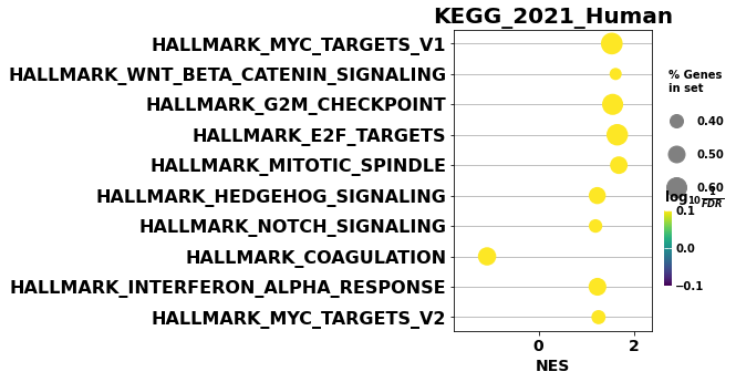
[53]:
from gseapy import dotplot
# to save your figure, make sure that ``ofname`` is not None
ax = dotplot(gs_res.res2d,
             column="FDR q-val",
             title='KEGG_2021_Human',
             cmap=plt.cm.viridis,
             size=5,
             figsize=(4,5), cutoff=1)
2.5.3. Command line usage
You may also want to use gsea in command line
[54]:
# !gseapy gsea -d ./data/P53_resampling_data.txt \
#              -g KEGG_2016 -c ./data/P53.cls \
#              -o test/gsea_reprot_2 \
#              -v --no-plot \
#              -t phenotype
2.6. Single Sample GSEA example
What’s ssGSEA? Which one should I use? Prerank or ssGSEA
see FAQ here
Assign - data with - a txt file, gct file, - pd.DataFrame - pd.Seires(gene name as index)
gene_sets with:
gene_sets="KEGG_2016",
gene_sets="KEGG_2016,KEGG2013",
gene_sets="./data/genes.gmt",
gene_sets=["KEGG_2016","./data/genes.gmt"],
gene_sets={'A':['gene1', 'gene2',...],
           'B':['gene2', 'gene4',...],
           ...}
Gene symbols are all “UPCASES” in the Enrichr Libaries. You should convert your input gene identifier to “UPCASES” first.
If input
gmt,dictobject, please refer to1.2 Mouse gene symbols maps to Human, or Vice Versa(in this page) to convert gene identifier
[55]:
import gseapy as gp
# txt, gct file input
ss = gp.ssgsea(data='./tests/extdata/Leukemia_hgu95av2.trim.txt',
               gene_sets='./tests/extdata/h.all.v7.0.symbols.gmt',
               outdir=None,
               sample_norm_method='rank', # choose 'custom' will only use the raw value of `data`
               no_plot=True)
2023-10-25 10:46:59,844 [WARNING] Found duplicated gene names, values averaged by gene names!
[56]:
ss.res2d.head()
[56]:
| Name | Term | ES | NES | |
|---|---|---|---|---|
| 0 | ALL_2 | HALLMARK_MYC_TARGETS_V1 | 3393.823575 | 0.707975 |
| 1 | ALL_12 | HALLMARK_MYC_TARGETS_V1 | 3385.626111 | 0.706265 |
| 2 | AML_11 | HALLMARK_MYC_TARGETS_V1 | 3359.186716 | 0.700749 |
| 3 | ALL_14 | HALLMARK_MYC_TARGETS_V1 | 3348.938881 | 0.698611 |
| 4 | ALL_17 | HALLMARK_MYC_TARGETS_V1 | 3335.065348 | 0.695717 |
[57]:
# or assign a dataframe, or Series to ssgsea()
ssdf = pd.read_csv("./tests/data/temp.rnk", header=None,index_col=0,  sep="\t")
ssdf.head()
[57]:
| 1 | |
|---|---|
| 0 | |
| ATXN1 | 16.456753 |
| UBQLN4 | 13.989493 |
| CALM1 | 13.745533 |
| DLG4 | 12.796588 |
| MRE11A | 12.787631 |
[58]:
# dataframe with one column is also supported by ssGSEA or Prerank
# But you have to set gene_names as index
ssdf2 = ssdf.squeeze()
[59]:
# Series, DataFrame Example
# supports dataframe and series
temp  = gp.ssgsea(data=ssdf2, gene_sets="./tests/data/temp.gmt")
2.6.1. Access Enrichment Score (ES) and NES
Results are saved to obj.res2d
[60]:
# NES and ES
ss.res2d.sort_values('Name').head()
[60]:
| Name | Term | ES | NES | |
|---|---|---|---|---|
| 601 | ALL_1 | HALLMARK_PANCREAS_BETA_CELLS | -1280.654659 | -0.267153 |
| 934 | ALL_1 | HALLMARK_APOPTOSIS | 970.818772 | 0.202519 |
| 1774 | ALL_1 | HALLMARK_HEDGEHOG_SIGNALING | 431.446694 | 0.090003 |
| 279 | ALL_1 | HALLMARK_INTERFERON_ALPHA_RESPONSE | 1721.458034 | 0.359108 |
| 1778 | ALL_1 | HALLMARK_BILE_ACID_METABOLISM | -429.127871 | -0.089519 |
[61]:
nes = ss.res2d.pivot(index='Term', columns='Name', values='NES')
nes.head()
[61]:
| Name | ALL_1 | ALL_10 | ALL_11 | ALL_12 | ALL_13 | ALL_14 | ALL_15 | ALL_16 | ALL_17 | ALL_18 | ... | AML_22 | AML_23 | AML_24 | AML_3 | AML_4 | AML_5 | AML_6 | AML_7 | AML_8 | AML_9 |
|---|---|---|---|---|---|---|---|---|---|---|---|---|---|---|---|---|---|---|---|---|---|
| Term | |||||||||||||||||||||
| HALLMARK_ADIPOGENESIS | 0.287384 | 0.274548 | 0.290059 | 0.285388 | 0.322757 | 0.305239 | 0.275686 | 0.266209 | 0.315803 | 0.282617 | ... | 0.277755 | 0.261477 | 0.200083 | 0.312948 | 0.342963 | 0.253282 | 0.298924 | 0.410395 | 0.387433 | 0.343606 |
| HALLMARK_ALLOGRAFT_REJECTION | 0.06177 | 0.028062 | 0.096589 | 0.080713 | 0.082701 | 0.102735 | 0.12525 | 0.147262 | 0.124621 | 0.091077 | ... | 0.185738 | 0.157852 | 0.055585 | 0.218827 | 0.172395 | 0.199077 | 0.158945 | 0.13835 | 0.110787 | 0.121643 |
| HALLMARK_ANDROGEN_RESPONSE | 0.133453 | 0.113911 | 0.193074 | 0.201531 | 0.151001 | 0.12967 | 0.173563 | 0.144836 | 0.180214 | 0.180801 | ... | 0.180443 | 0.188891 | 0.197979 | 0.174892 | 0.14285 | 0.184843 | 0.157449 | 0.162843 | 0.180475 | 0.181878 |
| HALLMARK_ANGIOGENESIS | -0.113481 | -0.182411 | -0.195637 | -0.094817 | -0.163717 | -0.139243 | -0.119084 | -0.154526 | -0.06829 | -0.121156 | ... | 0.054883 | -0.023782 | 0.119022 | -0.067741 | 0.04843 | 0.012808 | 0.032505 | -0.024058 | -0.039492 | -0.043769 |
| HALLMARK_APICAL_JUNCTION | 0.051372 | 0.063763 | 0.054601 | 0.014385 | 0.049019 | 0.05269 | 0.064787 | 0.052192 | 0.05607 | 0.064936 | ... | 0.10927 | 0.090065 | 0.155801 | 0.091556 | 0.110045 | 0.101659 | 0.128808 | 0.095511 | 0.080076 | 0.098644 |
5 rows × 48 columns
Warning !!!
if you set permutation_num > 0, ssgsea will become prerank with ssGSEA statistics. DO NOT use this, unless you known what you are doing !
ss_permut = gp.ssgsea(data="./tests/extdata/Leukemia_hgu95av2.trim.txt",
               gene_sets="./tests/extdata/h.all.v7.0.symbols.gmt",
               outdir=None,
               sample_norm_method='rank', # choose 'custom' for your custom metric
               permutation_num=20, # set permutation_num > 0, it will act like prerank tool
               no_plot=True, # skip plotting, because you don't need these figures
               processes=4, seed=9)
ss_permut.res2d.head(5)
2.6.2. Command line usage of ssGSEA
[62]:
# !gseapy ssgsea -d ./data/testSet_rand1200.gct \
#                -g data/temp.gmt \
#                -o test/ssgsea_report2  \
#                -p 4 --no-plot
3. GSVA example
[63]:
import gseapy as gp
# txt, gct file input
es = gp.gsva(data='./tests/extdata/Leukemia_hgu95av2.trim.txt',
             gene_sets='./tests/extdata/h.all.v7.0.symbols.gmt',
             outdir=None)
2023-10-25 10:47:01,160 [WARNING] Found duplicated gene names, values averaged by gene names!
[64]:
es.res2d.pivot(index='Term', columns='Name', values='ES').head()
[64]:
| Name | ALL_1 | ALL_10 | ALL_11 | ALL_12 | ALL_13 | ALL_14 | ALL_15 | ALL_16 | ALL_17 | ALL_18 | ... | AML_22 | AML_23 | AML_24 | AML_3 | AML_4 | AML_5 | AML_6 | AML_7 | AML_8 | AML_9 |
|---|---|---|---|---|---|---|---|---|---|---|---|---|---|---|---|---|---|---|---|---|---|
| Term | |||||||||||||||||||||
| HALLMARK_ADIPOGENESIS | -0.21331 | -0.08096 | 0.003289 | -0.017909 | 0.207841 | 0.023294 | -0.085392 | -0.221273 | 0.16147 | -0.01825 | ... | 0.03344 | -0.190436 | -0.0985 | 0.105208 | 0.196799 | -0.296305 | -0.084042 | 0.450832 | 0.226921 | 0.209835 |
| HALLMARK_ALLOGRAFT_REJECTION | -0.210468 | -0.373787 | -0.086016 | -0.169623 | -0.158775 | -0.016488 | -0.050703 | 0.10443 | -0.075816 | -0.193654 | ... | 0.023653 | 0.032892 | -0.113577 | 0.30703 | 0.134581 | 0.188905 | 0.132169 | 0.024078 | -0.092054 | -0.195987 |
| HALLMARK_ANDROGEN_RESPONSE | -0.13633 | -0.308572 | 0.008126 | 0.04849 | -0.061181 | -0.203036 | 0.070416 | -0.12524 | 0.080075 | 0.022248 | ... | 0.031898 | 0.064394 | 0.070232 | 0.199349 | -0.079399 | -0.016658 | -0.127327 | 0.018847 | 0.121426 | 0.163149 |
| HALLMARK_ANGIOGENESIS | 0.035895 | -0.287645 | -0.214951 | -0.291145 | -0.311917 | -0.236717 | -0.345662 | -0.250202 | -0.233296 | -0.318353 | ... | 0.244374 | -0.076852 | -0.010928 | -0.210787 | 0.387912 | 0.269447 | 0.34823 | 0.157249 | 0.075479 | -0.064515 |
| HALLMARK_APICAL_JUNCTION | -0.088652 | -0.128757 | -0.050282 | -0.248682 | -0.145164 | 0.001997 | -0.082962 | -0.091691 | -0.168941 | -0.139766 | ... | 0.005859 | -0.067385 | 0.062719 | -0.022434 | 0.076593 | 0.138664 | 0.240647 | 0.039307 | 0.016764 | 0.057512 |
5 rows × 48 columns
[65]:
# !gseapy ssgsea -d ./tests/data/expr.gsva.csv \
#                -g ./tests/data/geneset.gsva.gmt \
#                -o test/gsva_report
3.1. Replot Example
3.1.1. Locate your directory
Notes: replot module need to find edb folder to work properly. keep the file tree like this:
data
 |--- edb
 |    |--- C1OE.cls
 |    |--- gene_sets.gmt
 |    |--- gsea_data.gsea_data.rnk
 |    |--- results.edb
[66]:
# run command inside python console
rep = gp.replot(indir="./tests/data", outdir="test/replot_test")
3.1.2. Command line usage of replot
[67]:
# !gseapy replot -i data -o test/replot_test